Objectives of the tutorial
The objective of this tutorial is to enable you to use the basic functionalities of Stambia.
We will address the following points:
- Project creation
- Metadata creation and reverse
- Mapping creation
- Process creation and execution
We will be handling the following technologies:
- Databases
- Flat files
Starting the tutorial environment
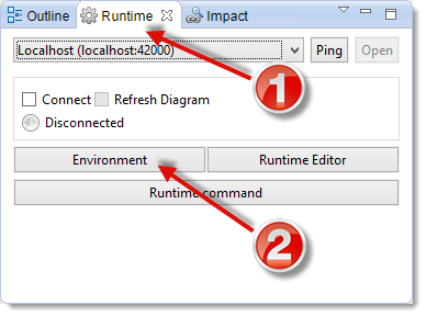
Open the Environment dialog box which is in the runtime view.
Information: The word view will often be used in this document and refers to the repositionable windows of Stambia Designer. In Stambia Designer, views are found around the central area (otherwise called edition area) where the different files are opened. Some of these views synchronize their content according to the object that is selected in the central area, or in the Project Explorer.
Now click on the buttons Start local Runtime and Start demo Databases.
- The button Start local Runtime allows you to launch a local Runtime on your machine.
This runtime will be used for managing the execution of your developments. We will see in another tutorial that you can also manually launch a Runtime and control all the launching parameters, and even start it as a Windows Service.
- The button Start demo Databases allows you to launch light demonstration databases on your machine that will be used for this tutorial.
Finally, click on Connect.
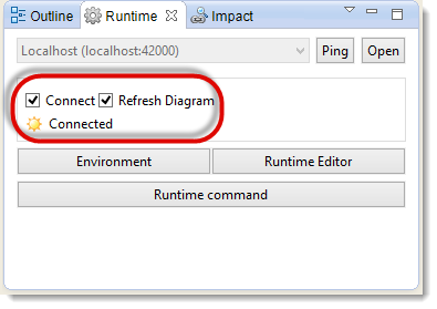
Checking Connect tells your Designer it has to connect to the Runtime.
Checking Refresh Diagram tells the Designer to show you the results of the executions (statistics, variables, colors, statuses...) in real-time.
Your Designer must be connected to a Runtime in order to be able to execute the Processes that you will develop.
Tip:
If you stop the demo environment or if you stop your machine, do not forget to restart the demo environment before you resume work on the tutorial at the place where you stopped.
Important:
Be careful to stop properly the demo databases when closing the environment, with the use of the Stop demo Databases button.
Closing them violently may lead to the instability of the demo databases.
If you are facing instabilities with it, if the connection is running indefinitely, or if you dropped or remove by mistake tables or data, you can at any time re-initialize the demo environment.
For this refer to the following article:
Reset tutorials demo databases
Creation of the tutorial Project
What is a project?
A Project is a container where you can organize and group a coherent set of developments in one place.
In fact, a Project is a physical directory which can be found inside the workspace.
All the files contained in the Project are physically stored in a directory tree. This means they can be archived and handled just like standard system files or folders.
Creation of the Project
Create this tutorial’s Project:
- Go to the Project Explorer view
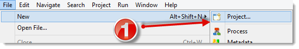
- Click on the File menu, then New and finally Project...
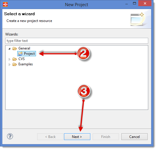
- In the window Select a Wizard, unfold the node General, then select Project
- Click on the button Next
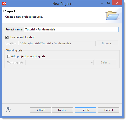
- Now give a name to your project. In the Project name box, set the value
Tutorial - Fundamentals - Click on Finish
Creation of the first Metadata
What is a Metadata?
Stambia is based on  Metadata which enable it to design, generate and execute data integration Processes. For example, the structure of the tables, of the flat files or the XML files used in the data integration flows is defined as Metadata.
A Metadata file managed by Stambia usually represents a data model such as a database server or a folder with tables or files.
You can create a Metadata file by connecting to the database server, to the file system, etc. and by fetching the structure of the tables, files, etc. This operation is called a reverse-engineering.
Finally, in Stambia, the basic element of these Metadata files (also used as a source and/or a target of a Mapping) is called a Datastore. Each table, file, etc. corresponds to a Datastore.
In this section, you will learn how to create a Metadata file, and how to do a Reverse-engineering in order to fetch the definition of each of the Datastores.
Reversing the target database
Creation of the Metadata file
The target model is the database that corresponds to the Datamart which is one of the two bases you have started before.
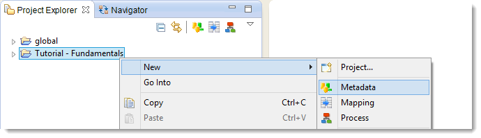
- In the Project Explorer view, right click on the Project Tutorial – Fundamentals
- Choose New then Metadata...
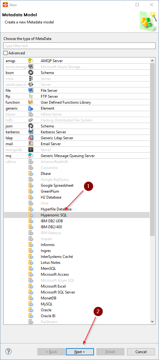
Stambia optimizes the flows depending on the underlying technology, but can also suggest relevant metadata for each technology. This is why you have to choose the type of Metadata you are creating. In the present case, the Datamart database is a Hypersonic SQL base (one of the two bases of the demonstration environment).
In the list that opens, choose  Hypersonic SQL then click on Next.
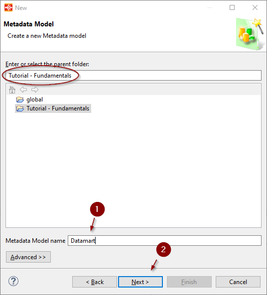
Enter Datamart in the Metadata Model name box then click on Next.
You will notice that the parent Folder’s name is already filled in with the name of the Project.
If you had not created the Metadata file by right-clicking on the Project, you would have had to choose the parent Folder Tutorial – Fundamentals.
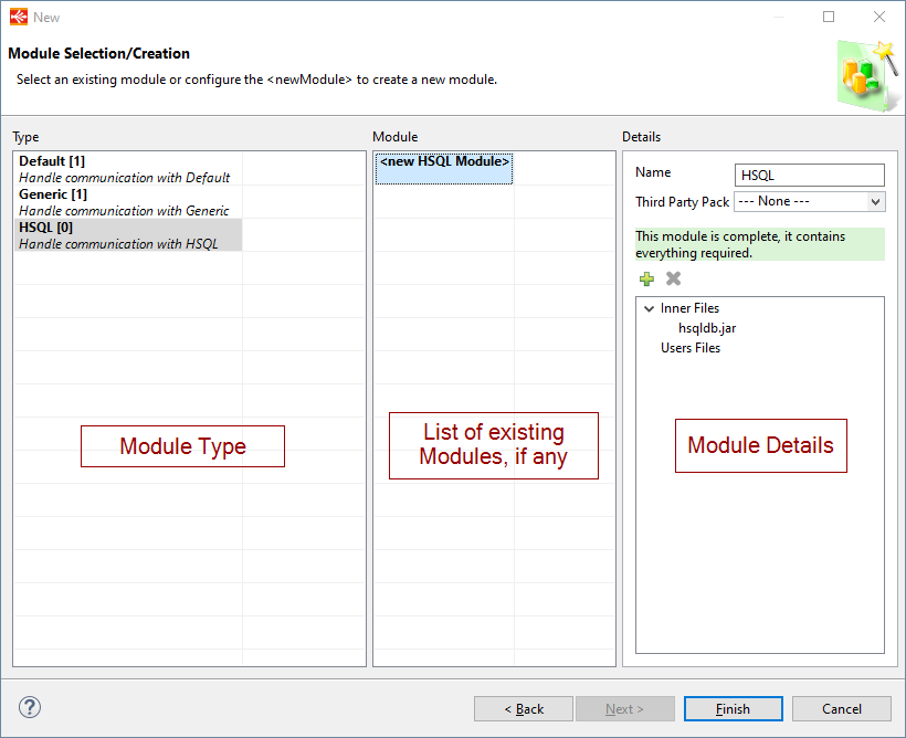
Next step is the selection of a Module, which will handle communication with HSQL demo database.
A Module is a set of one or multiple files which are necessary for the communication with databases.
As we are here creation an HSQL Metadata to connect to an HSQL demo database, the assistant is therfore proposing to create a new HSQL Module, or to select an existing one, if any.
Stambia ships everything required to communicate with HSQL: the JDBC driver «hsqldb.jar».
You can therefore click on Finish to finalize Metadata and Module creation.
From this moment, the Metadata file is created and Stambia automatically opens the Dataserver Assistant in order to define it. This assistant will then do with you the Reverse engineering in order to fetch the definition of the tables of this database.
Definition of the database Server
- Enter the JDBC URL of the database Server:
jdbc:hsqldb:hsql://localhost:62211 - Enter the User that corresponds to the username needed to connect to the database:
sa - Click on Connect
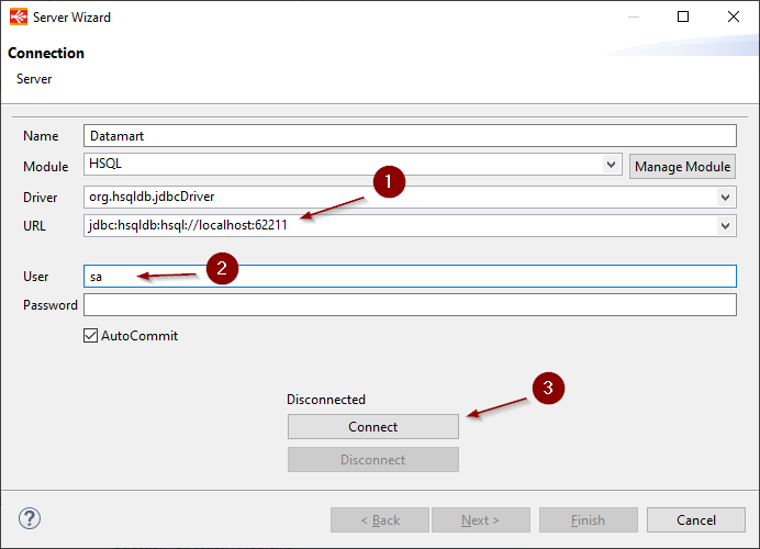
Stambia Designer then opens a JDBC connection to the database and the Next button will become available. Click on it to access the Schema definition window.
Definition of the Schema
- Click on the button Refresh Values so that Stambia Designer can fetch the list of the available schemas in this database.
- Select the Schema Name
HOTEL_DATAMART. - Click on Next to access the window where you will select the Datastores you wish to reverse.
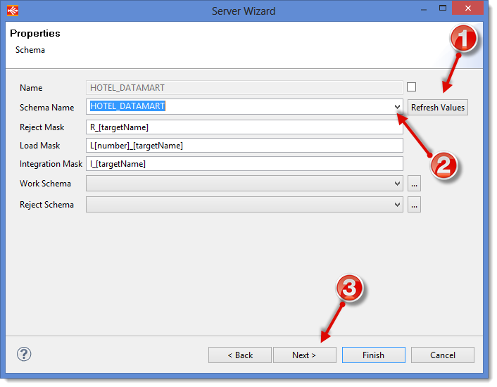
Information: To make this tutorial easier, the Work Schema and the Reject Schema are left empty, which means the technical tables generated by Stambia will be directly stored in the
HOTEL_DATAMARTschema. However, when using Stambia, it is recommended that you provide separate schemas for the work tables and the reject tables.
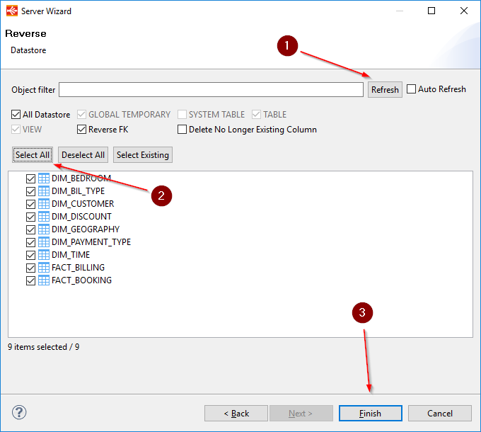
You can now select the tables in the HOTEL_DATAMART Schema that you wish to reverse.
Reversing the tables
- Click on the Refresh button to load the tables that are available for the Reverse.
- Click on the Select all button in order to reverse all the tables in this schema.
- Click on Finish to launch the reversing of the tables
Saving the Metadata file
You have now come back to the window where you can edit the Metadata file.
Notice the asterisk next to the name of the Metadata file:
This asterisk shows that the Metadata file has been changed but not saved. Before moving on, you will have to save this file so that Stambia Designer uses the right file content.
Click on the icon  or type CTRL+S on your keyboard in order to save y=the file.
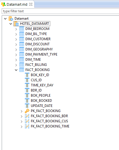
Exploring the reversed tables
If you wish to get to know the data of this model, you can use Stambia Designer to view the structure of the tables you have just reversed:
- Unfold the node of the Data server Datamart
- Then unfold the node of the HOTEL_DATAMART schema you have just reversed
You can now see all the tables that you had selected for the Reverse engineering in Stambia Designer as Datastores.
If you now unfold the node corresponding to each of the Datastores, you have access to their structure: columns, primary key, foreign keys, etc.
Reversing a delimited file
Creation of the Metadata file
Create another Metadata file with the following characteristics:
- Location: in the Tutorial – Fundamentals Project
- Metadata Model name: Reference Files
- Metadata Type: File Server
Once you have clicked on Finish, the assistant opens. Notice that this assistant is not the same as the one you used to create a Metadata file for a database.
Definition of the folder containing the file
- Fill in the field Name with the value Reference Files Folder.
- Now click on Browse, then browse to reach the directory where Stambia has been installed. Continue to browse the stambiaRuntime directory, then samples. Here, select the files directory
- Click on Next
Information: Notice that the Name we give here to the directory does not correspond to the physical name of the directory we are selecting (here files). This allows Stambia to use a name that means something to the user, while the physical name may be more complicated. You will also see in another tutorial how Stambia allows you to link different physical values to a same logical folder name.
You will now reach the window where you can define the file’s structure.
Defining the file’s structure
- Click on Browse and select the
DiscountRanges.txtfile - Check that the Type is DELIMITED because the
DiscountRanges.txtfile is a file with field separators. - The
DiscountRanges.txtfile contains fields that are separated by commas. In the field Field Separator select,
You can now click on Refresh in order to have a preview of the file’s content. In this preview, you can see that the file has got a first line with the name of each field.min,max,range0,9,0-910,19,10-1920,29,20-2930,39,30-3940,49,40-4950,100,more than 50
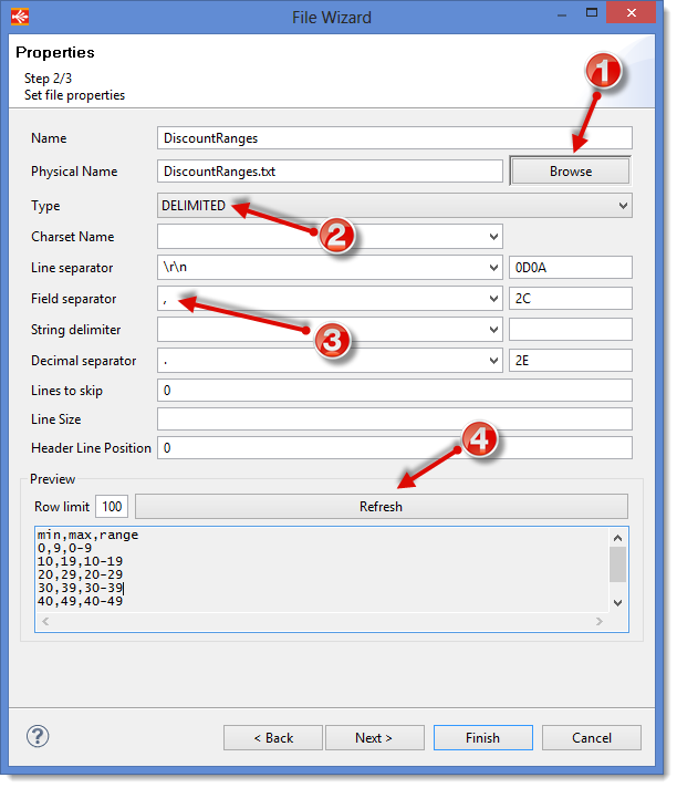
In order to tell Stambia Designer to use the first line of the file to name the columns, put 1 in the Header Line Position field.
If you click again on Refresh you will see that the first line is no more a part of the data read by Stambia:0,9,0-910,19,10-1920,29,20-2930,39,30-3940,49,40-4950,100,more than 50
Click on Next to access Datastore columns definition.
Defining the columns of the file
Click on Reverse in order to launch the Reverse engineering of the file’s columns.
Check that the columns are correctly defined with the following properties:
| Name | Position | Type |
|---|---|---|
| min | 1 | Numeric |
| max | 2 | Numeric |
| range | 3 | String |
You can check if the file definition is correct by clicking on Refresh in order to see how the data are interpreted by Stambia.
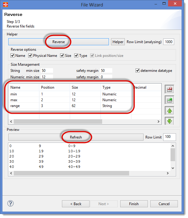
Click on Finish to finish the definition of this Datastore.
Saving the Metadata file
Do not forget that at this stage, the Metadata file hasn’t yet been saved.
Click on the icon or type CTRL+S on your keyboard to save the file.
Viewing the file data
Stambia Designer allows easy access to the datastores data so you can check how they are read by Stambia:
- Unfold the Server node then the Reference Files Folder node
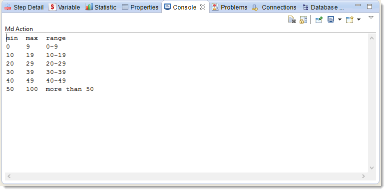
- Right-click on DiscountRanges then choose Actions and finally Consult Data (console)
Check the data shown in the Console view. They are shown in the form of columns separated by tabulations and the first line is the name of the columns.
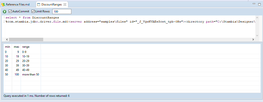
Stambia Designer also includes a component that allows you to visualize these data using a SQL query:
- Right-click on DiscountRanges then choose Actions and finally Consult Data
- The SQL query editor will now open with the request that will allow you to consult the file’s data.
- Click on
 or press CTRL+Enter
Warning: Data consultation is based on the Metadata file. If this file has not been saved, you will not be able to consult the data of your datastore.
Templates
What is a Template?
In order to generate data integration Processes, Stambia uses Templates which will generate Processes based on the business rules defined by the user.
In this way, the user concentrates on the «What» (business rules) while the template automatically manages the «How» (technical process).
All the business rules you defined will there be translated automatically into technical rules by Templates, which moreover have a bunch of options to customize behaviors if needed.
Designing the first Mapping
What is a Mapping?
A Mapping allows you to define the data transformation rules from one or more source Datastores in order to load one or more target Datastores. These business rules will then be used by the Templates of this Mapping in order to generate a complete and optimized data integration Process.
Creating a simple Mapping
Creating the Mapping that loads DIM_DISCOUNT table
Start by creating the Mapping file which will be used to load the table DIM_DISCOUNT:
- In the Project Explorer view, right-click on the Tutorial – Fundamentals Project
- Choose New then
 Mapping...
Enter Load DIM_DISCOUNT in the File name field then click on Finish.
Tip: You will notice that the Parent Folder name is already filled in with the name of the Project. If you hadn’t created the Mapping file by a right-click on the Project, you would have had to choose the Parent Folder.
From this moment, the Mapping file has been created and the editor opens so that you can start defining the transformation.
Adding datastores to the Mapping
The first step consists in adding the required datastores to the mapping:
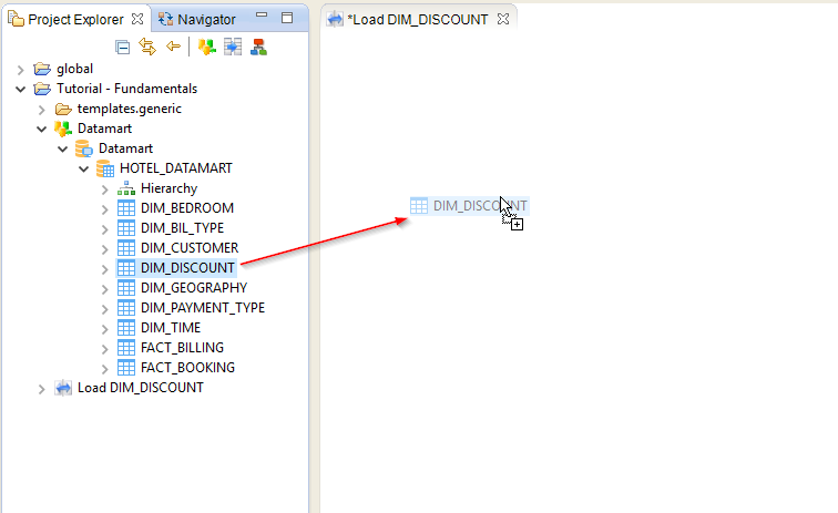
- In the Project Explorer view, unfold the node of the Tutorial – Fundamentals project
- Then unfold the node of the Datamart Metadata file.
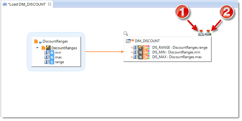
Inside this arborescence, find the DIM_DISCOUNT datastore. Drag and drop this Datastore from the Project Explorer view to the editor of the Load DIM_DISCOUNT Mapping.
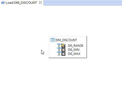
Repeat this operation for the next Datastore: DiscountRanges.
- Drag and drop the DiscountRanges Datastore which can be found in the Metadata file Reference Files
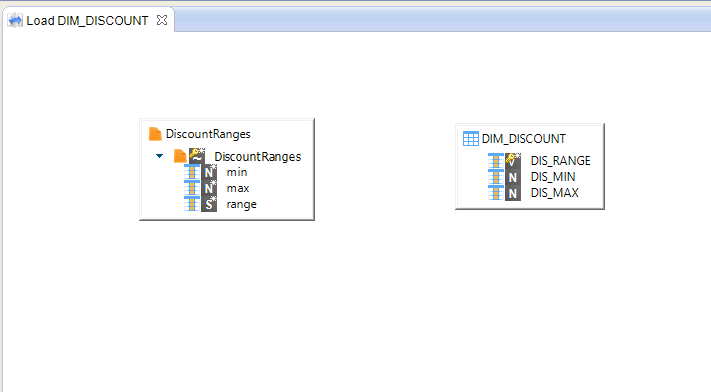
The object of this mapping is to load DIM_DISCOUNT with the data found in the DiscountRanges file.
DIM_DISCOUNT is the "Target" Datastore (that is to be loaded) and DiscountRanges the "Source" Datastore.
Information: In a mapping, each Datastore can be a target and/or a source.
Defining expressions
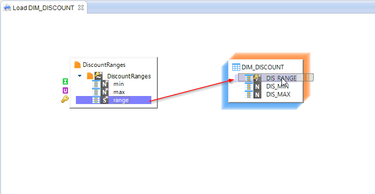
We now need to define the transformation expressions. These expressions have to be defined for each column loaded by the Mapping.
In this first Mapping, the expression are simple:
| Target column | Expression |
|---|---|
| DIS_RANGE | DiscountRanges.range |
| DIS_MIN | DiscountRanges.min |
| DIS_MAX | DiscountRanges.max |
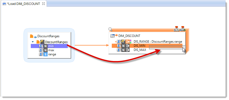
You will see further on in this tutorial how to define more complex expressions. For this Mapping, you can simply drag and drop each source column directly on the matching target column. Stambia Designer will then define the corresponding expression.
On your first drag-and-drop, Stambia Designer will ask you which type of relationship you want to define between the two Datastores: select Map.
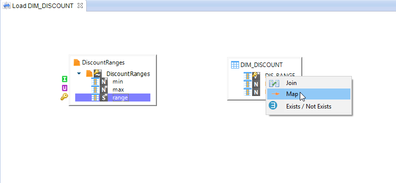
Repeat for the other columns. Stambia Designer will not ask you which type of relationship you want since it has already been specified.
Integration and Load Steps
- Stambia Designer detects that the source (a file) and the target (a table in a database) are stored with different technologies and automatically adds a Load step. This new step will help define and configure the Template that will be used to load the source into the target database. For this Mapping, you can use the default values.
- Stambia Designer automatically adds an Integration step which allows you to define the Template you will be using to integrate the data into this target and to configure it. For this Mapping, you can use the default values (we will see with other Mappings further on in this tutorial how to configure a Load Template).
The Runtime
The Mapping you just created is now ready to be executed.
Every execution is handled by the Runtime software, which job is to execute all the tasks planned by the user in the Mapping: here loading a target table from a source file.
This is the utility you started in the Starting the tutorial environment step.
To be able to execute your first Mapping, it is necessary to restart the Runtime to take into account the new HSQL Module created while creating your first Metadata.
This is necessary only when creating new Modules in Runtime, as they are taken into account at its startup.
If you start a Runtime already containing Modules, you can use them at execution right away.
A Module having the purpose to be reused, it is most commonly created once and then reused in all applicable Metadata.
For instance, the HSQL Module created during the tutorial can be used for all connections to HSQL databases. By the way, it will be reused later in this tutorial.
Restarting the Runtime
To restart the Runtime, the procedure is similar to the one you followed for starting it.
In Runtime View, open the «Environment» dialog box and then click on Stop Local Runtime.
Finally, click on Start Local Runtime to start it again.
You can then close this window by clicking on OK, and waits for the Designer to reconnect to the Runtime.
Do not forget to check the «Connect» box if it is not already checked.
Executing the first Mapping
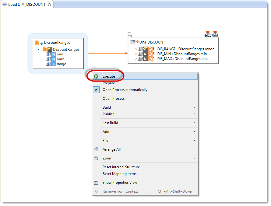
The Mapping is now finished. To execute it:
- Start by saving it.
- Then right-click on the background of this mapping’s diagram.
- Click on Execute
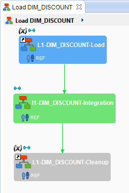
Stambia Designer will launch the execution of this Mapping and open a new window that shows the Process that was generated thanks to the Templates and the business rules you defined in the Mapping. In this window, you can follow the Mapping’s execution:
- The steps colored in grey are the steps waiting to be executed
- Les steps colored in green are currently being executed
- Les steps colored in blue are finished with success
- Les steps colored in red are finished but failed
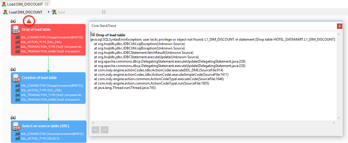
Warning: Do not forget to check that the Runtime did start and that you are connected to it. If you are not sure, turn to the section Starting the environment
Information: If an error occurs during the execution of a Process, an additional icon is displayed. Click on this icon in order to display the full stack trace of the error. If the error indicates that HSQL Module does not exist or cannot be found, check that you have properly restarted your Runtime before creating HSQL module during Creation of the first Metadata step. Creating a new Module requires the Runtime to be restarted, as indicated in Runtime section of this tutorial.
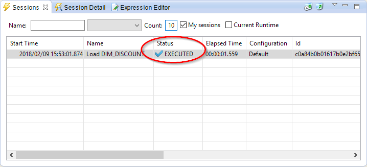
Analyzing the result of the execution
The execution of this Mapping by Stambia produced a Session which was executed on the Runtime.
We will start by checking the status of the Session in the Sessions view.
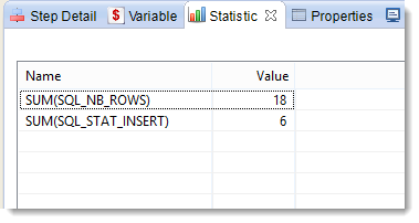
You can also see the execution statistics in the Statistic view. This view lists the following:
| Name | Value |
|---|---|
SUM(SQL_NB_ROWS) |
18 |
SUM(SQL_STAT_INSERT) |
6 |
SUM(SQL_STAT_UPDATE) |
0 |
We can see that a total of 18 lines were handled, and that 6 lines were inserted.
If you execute the Mapping once more, you will notice that the statistics will change:
| Name | Value |
|---|---|
SUM(SQL_NB_ROWS) |
18 |
SUM(SQL_STAT_INSERT) |
0 |
SUM(SQL_STAT_UPDATE) |
0 |
The number of inserted lines now changes to 0 because they were already inserted during the previous execution.
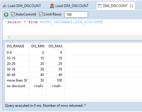
We can now check if the data were correctly inserted into the target table:
- In the Mapping window, right-click on the target datastore (DIM_DISCOUNT) and select Action then Consult data
- The SQL request editor opens and you can execute the request by clicking on or by typing CTRL+Enter
Creating other Metadata
In order to continue with this tutorial, you must now define all the data sources that will be used.
Reversing the source model
This tutorial uses another Hypersonic SQL database which will be used as a source for several Mappings. Create the corresponding Metadata file and do the reverse engineering using the following properties:
| Property | Value |
|---|---|
| Location | Create the Metadata file directly in the Tutorial – Fundamentals Project |
| Technology | Hypersonic SQL |
| Metadata Model name | Hotel |
| URL | jdbc:hsqldb:hsql://localhost:62210 |
| User | sa |
| Password | |
| Schema | HOTEL_MANAGEMENT |
For the other properties, you will use the default values.
Tip: If you have difficulties, you can always refer to the procedure we followed in the section Reversing the target model
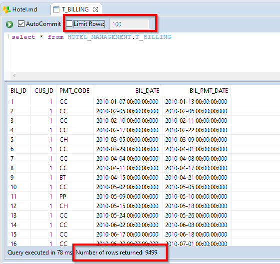
You can then get to know the data of this database with a right-click on each datastore, selecting Actions then Consult data.
Warning: Some tables contain a lot of lines (particularly the tables T_BDR_PLN_CUS, T_BILLING, T_BILLING_LINES and T_PLANNING). By default, Stambia Designer limits to 100 the number of lines you can read in order to avoid performance problems with very big tables. If you want to see all the data contained in these tables, uncheck the Limit Rows box.
Reversing the other delimited files
Since you have already defined the folder containing the flat files for this tutorial, you will not need to recreate a new Metadata file:
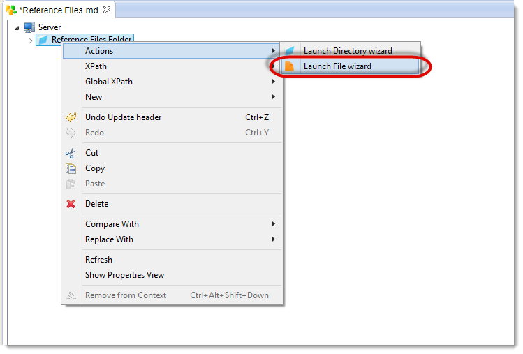
- Double-click on the Reference Files file
- Unfold the server node
- Right-click on Reference Files Folder and select Actions then Launch File wizard
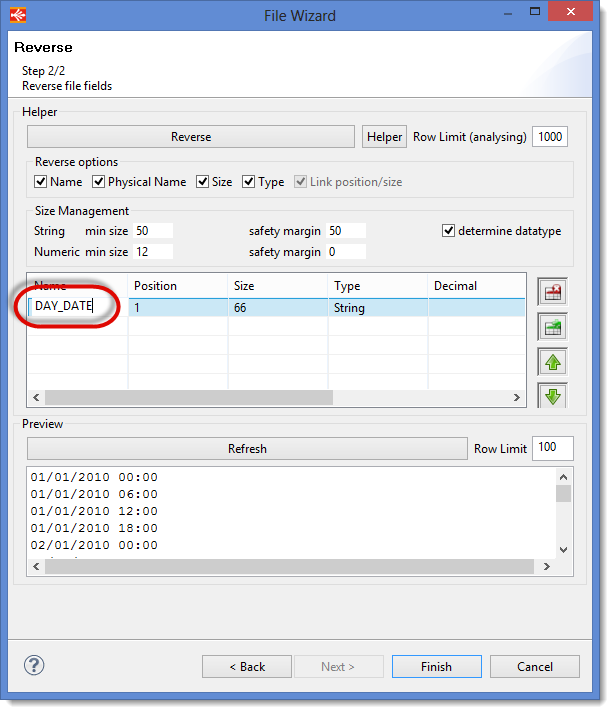
Reversing the file Time.csv
Define a delimited file with the following properties:
| Property | Value |
|---|---|
| Physical Name | Time.csv |
| Header Line Position | 0 |
This file will then have the following columns:
| Name | Position | Type |
|---|---|---|
| DAY_DATE | 1 | String |
To rename the column, start by doing the reverse, then change the name directly in the table.
Once you have finished declaring the file, you can check the data as they are seen by Stambia.
Tip: Do not forget to save the Metadata file before you consult the data.
Reversing the file REF_US_STATES.csv
Define a delimited file with the following properties:
| Property | Value |
|---|---|
| Physical Name | REF_US_STATES.csv |
| Field Separator | , |
| Header Line Position | 1 |
| Name | US_States |
Tip: You will notice that the datastore name is automatically filled in with the name of the file without the extension. You can manually change this name if you wish to use a more understandable or readable functional name: US_States.
This file will then have the following columns:
| Name | Position | Type |
|---|---|---|
| STATE_UPPER_CASE | 1 | String |
| STATE | 2 | String |
| STATE_CODE | 3 | String |
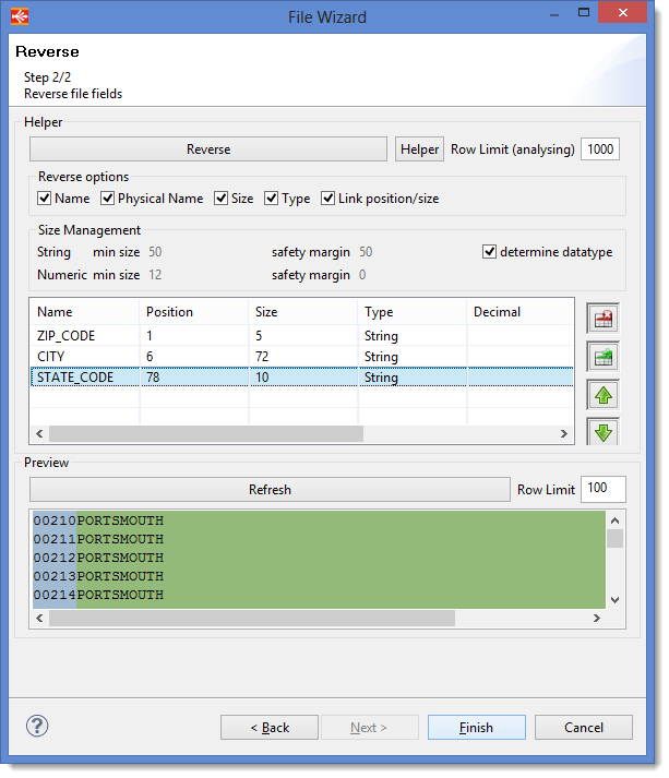
Reversing a positional file
A positional file is a flat file where the columns are not defined with a specific separator, but rather depending on the position of the characters. To create a positional file for this tutorial:
- Launch the File Reverse assistant
- Click on Browse and select the
ref_us_cities.txtfile - In the Name field, type: US_Cities
- Modify the Type and choose POSITIONAL
You can now check the content of the file by clicking on Refresh.
Click on Next to get to the window where you will define the columns.
In the case of a positional file with contiguous columns, the Reverse button cannot detect the different columns. You will have to define the columns manually. For each column in the following table:
- Click on
 to declare a new column
 - Change the properties of the column in the table
| Name | Position | Size | Type |
|---|---|---|---|
| ZIP_CODE | 1 | 5 | String |
| CITY | 6 | 72 | String |
| STATE_CODE | 78 | 10 | String |
Warning: Unlike delimited files where the position shows the number of the column, here, the position indicates the position of the first character of the column.
If you click on Refresh, you can preview the layout of the file.
Organizing the developments
Grouping the Metadata together in a project
As a general rule, Metadata files are shared by many Projects. So it is a good habit to group the metadata files in a dedicated Project, in order to manage and share them more easily.
Moreover, as part of these tutorials, some Metadata files will be shared with all the tutorials. Let us group these Metadata files into one Project:
- Create a Project:
Tutorial - Common Metadata - Drag and drop the Metadata Datamart file into the
Tutorial - Common MetadataProject
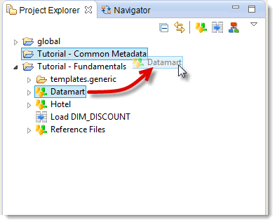
You can also use multiple selection to save time:
- Select Hotel
- While pressing CTRL key, select Reference Files
- Drag and drop the whole lot into the Tutorial – Common Metadata Project
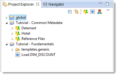
You now have a Project dedicated to Metadata:
Information: You can notice that reorganizing your files had no impact on the Load DIM_DISCOUNT Mapping. You can open it and execute it again as if nothing had changed. Reorganizing your developments is very easy with Stambia Designer.
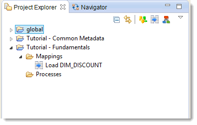
Grouping the developments with Folders
Create a Folder to group the Mappings:
- Right-click on the Tutorial – Fundamentals Project, select New then Folder
- Enter the name: Mappings
- Click on Finish
- Drag and drop the Load DIM_DISCOUNT Mapping into the Mappings Folder
In the same way, create a Processes Folder, which will be used a bit further on.
Creating a Mapping with a filter
Creating the Mapping that loads the DIM_PAYMENT_TYPE table
Create a new Mapping in the Mappings Folder with the following properties:
| Property | Value |
|---|---|
| Mapping name | Load DIM_PAYMENT_TYPE |
| Target Datastore | DIM_PAYMENT_TYPE |
| Source Datastore | T_PAYMENT_TYPE |
Tip: Remember that the Metadata files are now in the Tutorial – Common Metadata Project
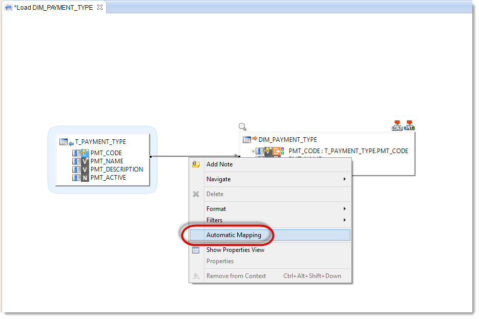
Tip: once you have defined at least one transformation expression between two datastores, Stambia Designer automatically maps the target and source columns that have the same name. If this is not the case, you can manually trigger the mapping of the various fields. To do this, start by displaying the links between datastores by clicking on the
icon in the toolbar. Then right-click on the link between the two datastores and select Automatic Mapping.
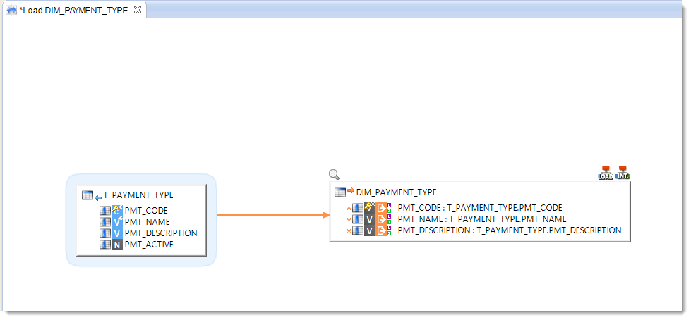
All the columns are now mapped:
Adding a filter
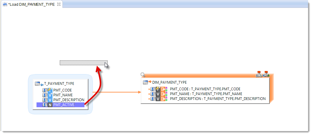
To load DIM_PAYMENT_TYPE we want to filter out the obsolete data found in the T_PAYMENT_TYPE table. The active data, meaning those we want to keep, are set apart by the PMT_ACTIVE column the value of which is set to 1. So we will create a Filter on the source Datastore:
- Drag and drop the PMT_ACTIVE column onto the background of the diagram
- Choose Create a Filter on the dialog box which opens
- Open the Expression Editor view
- Check that the expression of the filter is:
T_PAYMENT_TYPE.PMT_ACTIVE=1
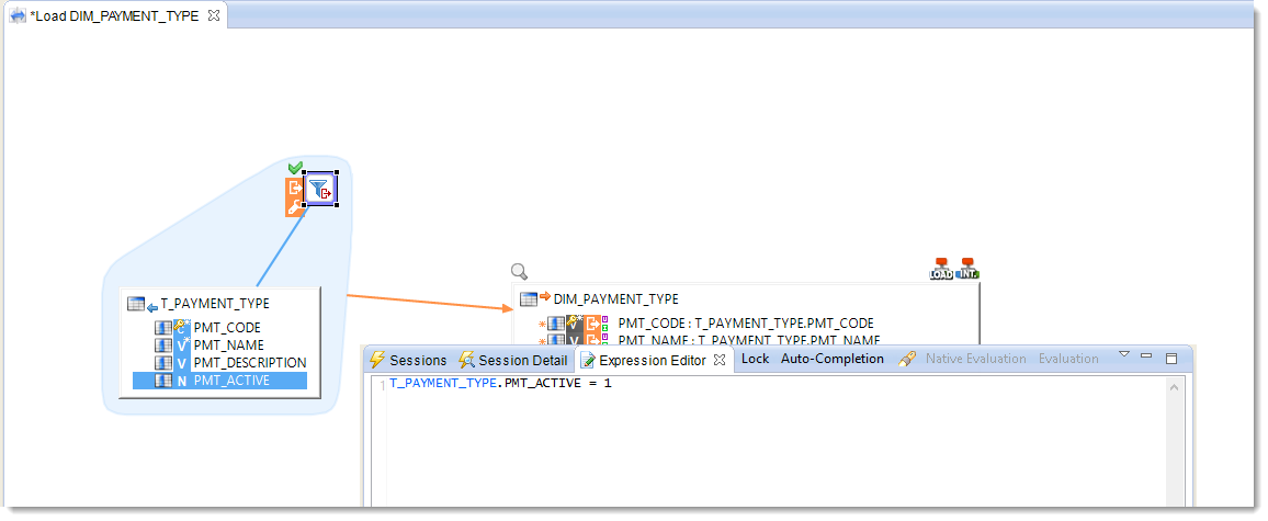
Information: Expression Editor View is located by default at the bottom of Designer, under the Mapping editor.
It is used to consult and modify the expressions of Mapping objects such as filter expressions, column expressions, ...
Executing the Mapping
The Mapping is now finished. To execute it:
- Start by saving it.
- Then right-click on the background of the diagram of this Mapping
- Click on Execute
Analyzing the result of the execution
Go to the Statistic view to check the statistics of this execution:
| Name | Value |
|---|---|
SUM(SQL_NB_ROWS) |
12 |
SUM(SQL_STAT_INSERT) |
4 |
SUM(SQL_STAT_UPDATE) |
0 |
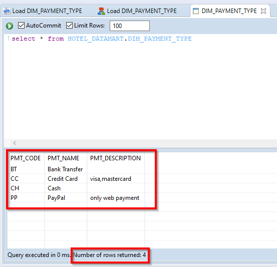
Check that the target table contains the 4 following lines:
| PMT_CODE | PMT_NAME | PMT_DESCRIPTION |
|---|---|---|
| BT | Bank Transfer | |
| CC | Credit Card | visa,mastercard |
| CH | Cash | |
| PP | PayPal | only web payment |
Information: If your data to not match the specifications hereabove, you probably didn’t properly define your filter. In order to reset the target table, you may start afresh with an empty table:
1. Right-click on the target Datastore: DIM_PAYMENT_TYPES
2. Select Action then Consult data
3. Now enter the following SQL command:delete from HOTEL_DATAMART.DIM_PAYMENT_TYPE
4. Click on
5. You can now correct your filter and launch again the execution
Discovering the generated code
Now come back to the window of the Process generated by Stambia Designer. This Process is composed of 3 blocks:
L1_DIM_PAYMENT_TYPE-LoadI1_DIM_PAYMENT_TYPE-IntegrationL1_DIM_PAYMENT_TYPE-Cleanup
Each block comes from a template used by the Load DIM_PAYMENT_TYPE Mapping.
The blocks L1_DIM_PAYMENT_TYPE-Load and L1_DIM_PAYMENT_TYPE-Cleanup come from the Template used for the Load step. L1_DIM_PAYMENT_TYPE-Load serves to transfer the data from the source table into the target database. As for L1_DIM_PAYMENT_TYPE-Cleanup, it is the steps to clean up temporary objects that might have been created during the execution of the L1_DIM_PAYMENT_TYPE-Load block.
If you double-click on the I1-DIM_PAYMENT_TYPE-Integration block to look at its contents, you will notice it consists of two blocks: I1-DIM_PAYMENT_TYPE-Prepare and I1-DIM_PAYMENT_TYPE-Integration.
The blocks I1-DIM_PAYMENT_TYPE-Prepare and I1-DIM_PAYMENT_TYPE-Integration come from the Template used for the Integration step. I1-DIM_PAYMENT_TYPE-Prepare serves for preliminary steps (creation of temporary objects, transformations of source data, etc.). And I1-DIM_PAYMENT_TYPE-Integration serves for the final integration of the data into the target table.
You may open each block to look into its content. Double-click on L1_DIM_PAYMENT_TYPE-Load. In this way, you can access the part of the Load Template which loads data into the target database. It is composed of Actions. Actions are the atomic elements used by Stambia during execution. The color code is the same as for the blocks of a higher level. You will also notice there are new colors:
- Steps colored in white have been ignored because they were useless in this Mapping
- Steps colored in yellow finished but failed, but these errors are tolerated by the template.
Now click on the Action Select on source table (SRC) and look at the code that was executed on the source base in the Step Detail view. You can especially notice that you can find the code that goes with the Filter you have created earlier in this Mapping.
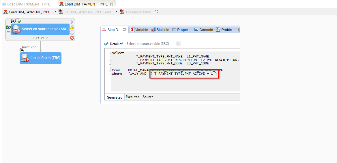
Information: The Source tab in the Step Detail view gives you access to the matching code that is in the Template but this is beyond the purpose of this tutorial.
Creating a Mapping with complex expressions
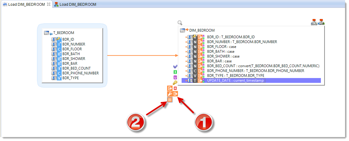
Creating the Mapping that loads the DIM_BEDROOM table
Create a new Mapping with the following properties:
| Property | Value |
|---|---|
| Parent folder | Mappings |
| Mapping name | Load DIM_BEDROOM |
| Target Datastore | DIM_BEDROOM |
| Source Datastore | T_BEDROOM |
Defining the business rules
Even if the source and target columns have the same name, we will have to do specific transformations to the data before they can be integrated into the target. For each column of the list herebelow:
- Click on the target column
- In the Expression Editor view, fill in the transformation expression
| Target column | Business rule |
|---|---|
| BDR_ID | T_BEDROOM.BDR_ID |
| BDR_NUMBER | T_BEDROOM.BDR_NUMBER |
| BDR_FLOOR | casewhen lower(T_BEDROOM.BDR_FLOOR) = 'gf' then 0when lower(T_BEDROOM.BDR_FLOOR) = '1st' then 1when lower(T_BEDROOM.BDR_FLOOR) = '2nd' then 2end |
| BDR_BATH | casewhen T_BEDROOM.BDR_BATH = 'true' then 1else 0end |
| BDR_SHOWER | casewhen T_BEDROOM.BDR_SHOWER = 'true' then 1else 0end |
| BDR_BAR | casewhen T_BEDROOM.BDR_BAR = 'true' then 1else 0end |
| BDR_BED_COUNT | convert(T_BEDROOM.BDR_BED_COUNT,NUMERIC) |
| BDR_PHONE_NUMBER | T_BEDROOM.BDR_PHONE_NUMBER |
| BDR_TYPE | T_BEDROOM.BDR_TYPE |
| UPDATE_DATE | current_timestamp |
You can execute the Mapping.
Analyzing the result of the execution
Got to the Statistic view to check the statistics of this execution:
| Name | Value |
|---|---|
SUM(SQL_NB_ROWS) |
60 |
SUM(SQL_STAT_INSERT) |
20 |
SUM(SQL_STAT_UPDATE) |
0 |
Optimizing the Mapping
If you execute once again this Mapping without changing the data, you will get the following new statistics:
| Name | Value |
|---|---|
SUM(SQL_NB_ROWS) |
80 |
SUM(SQL_STAT_INSERT) |
00 |
SUM(SQL_STAT_UPDATE) |
20 |
The 20 updated lines come from the UPDATE_DATE column whose value is the expression current_timestamp. By default, Stambia executes expressions on the source. This means that if you don’t do anything, for every data extraction from the source base, the UPDATE_DATE column will be extracted with a new value. Consequently, since the Mapping is by default in «incremental» mode (it compares the data), the update date will systematically differ from the one in the target, and will therefore be updated.
To avoid this, you are going to change the definition of the business rule linked to the UPDATE_DATE field and modify the transformation’s location for this field, so that it executes on the target. Because of this, the expression will be executed right at the end, and will thus be excluded from the comparison mechanism. To do the modification:
- Select the target column UPDATE_DATE
- Click on the
 icon in the Execution Location to the left of the Datastore.
 - Click on the
 icon meaning Target
Information: You can also modify the Execution Location via the Properties view or by right-clicking on the target column and selecting Execution Location then Target.
The Mapping is now optimized. You can execute it once more.
Tip: The transformation’s location will now be defined in the table specifying the transformation business rules in the column Execution location.
Analyzing the result of the execution
Go to the Statistic view to check the statistics of this execution:
| Name | Value |
|---|---|
SUM(SQL_NB_ROWS) |
60 |
SUM(SQL_STAT_INSERT) |
0 |
SUM(SQL_STAT_UPDATE) |
0 |
You can now see that the lines will be updated only if the source functional data have changed. The technical fields do not artificially inflate the data flow.
Creating a Mapping with joins
Creating the Mapping that loads the DIM_GEOGRAPHY table
Create a new Mapping with the following properties:
| Property | Value |
|---|---|
| Parent folder | Mappings |
| Mapping name | Load DIM_GEOGRAPHY |
| Target Datastore | DIM_GEOGRAPHY |
| Source Datastores | US_States, US_Cities |
The transformation business rules are:
| Target column | Business rule | Execution location |
|---|---|---|
| GEO_KEY_ID | next value for HOTEL_DATAMART.SEQ_GEO_KEY_ID |
Target |
| GEO_ZIP_CODE | US_Cities.ZIP_CODE |
Source |
| GEO_CITY | US_Cities.CITY |
Source |
| GEO_STATE_CODE | US_Cities.STATE_CODE |
Source |
| GEO_STATE | US_States.STATE_UPPER_CASE |
Source |
Warning: The business rule for the GEO_KEY_ID column uses here a sequence object that is native to the target database. As above, for the UPDATE_DATE column, you will have to execute this rule on the target, so as to avoid to overload uselessly the data flow.
Defining the functional key of the Mapping
The first step in defining this Mapping is to define the functional key. This key allows Stambia to identify a record in a unique way. Particularly, this functional key is used by Stambia to know if one of the source’s records has already been inserted into the target or if it is a new record.
By default, Stambia Designer relies on the Datastore’s primary key in order to automatically select a functional key. In the DIM_GEOGRAPHY table, the primary key is the GEO_KEY_ID column. Now, this column is loaded by a business rule that does not intervene in the source dataflow. This means that Stambia cannot rely on this column to recognize new and old records. So you will have to select another functional key for this Mapping:
- Select the GEO_KEY_ID column
- Click on the
 icon to disable the functional key on the column.
 - Then select the GEO_ZIP_CODE column
- Click on the icon to define it as functional key for the mapping.
The functional key that will be used by Stambia will now be the GEO_ZIP_CODE column. This means that, if a source record contains a GEO_ZIP_CODE value that does not exist in the target table, Stambia will create a new record. Likewise, if the GEO_ZIP_CODE value already exists in the target table, all the data of the record will be compared to the matching data in the target and updated if necessary with the new values from the source.
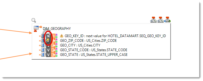
Information: You will notice that the icon symbolizing a key has moved from the GEO_KEY_ID column to the GEO_ZIP_CODE column. This helps you to quickly see which is the functional key of a Mapping.
Tip: The columns of the functional key will now be defined in the table specifying the transformation business rules in the column Characteristics.
Executing a business rule only for insertions
The target column GEO_KEY_ID is loaded by a database sequence. This object sends back a new value every time it is invoked. Now, let’s imagine that a town in the source file US_Cities had a typographical error, and that on the second execution, the mistake has been corrected in the file. If nothing is done, in this case, the dataflow will have a record for this town and will have to be updated. However, since the business rule is based on a sequence, this would mean giving a new identifier to the target record when it is updated.
To overcome this problem, this business rule should be applied only if there are insertions in the target (and not for updates):
- Select the GEO_KEY_ID column
- Click on the
 icon to disable the updating of the column.
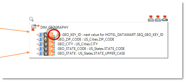
Information: You will notice that the icon with a
U(for Update) disappears. In this way, you can easily spot the business rules that are not executed during updates. As for the icon with anI(for Insert), it identifies the business rules that are activated for insertions.
Tip: The business rules required for the insertions or for the updates will now be defined in the table specifying the transformation business rules in the column Characteristics.
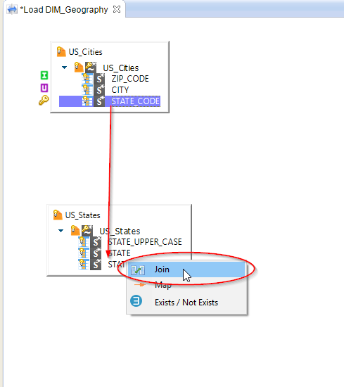
Defining the join between two source files
In the Mapping such as defined, the two data sets US_States and US_Cities are disjoint. Stambia would iterate the readings by combining all the lines of the first set with each line of the second set. You need to create a join between these two Datastores to avoid the Cartesian product:
- Drag and drop the STATE_CODE column from US_States to the STATE_CODE column in US_Cities.
- Check in the Expression Editor view that the business rule generated by Stambia Designer is correct.
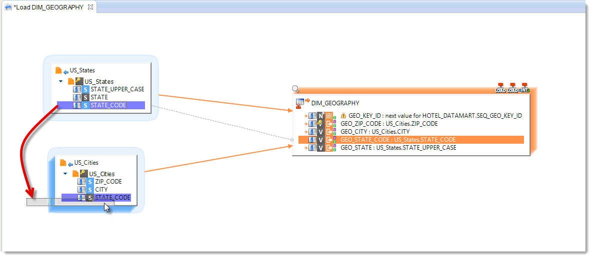
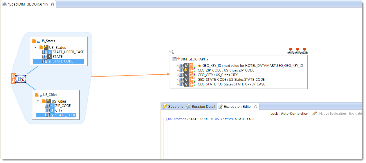
Important: Since the transformation business rules have already been defined on the target, the only possible relationship between the two Datastores US_States and US_Cities is a joint link. Stambia automatically creates the joint. If ever there was an ambiguity, a menu would pop up in which you would choose Join.
The Mapping is now finished, you can execute it.
Analyzing the result of the execution
Go to the Statistic view to check the statistics of this execution:
| Name | Value |
|---|---|
SUM(SQL_NB_ROWS) |
125 628 |
SUM(SQL_STAT_INSERT) |
41 693 |
SUM(SQL_STAT_UPDATE) |
0 |
If you execute this Mapping once more, your statistics become:
| Name | Value |
|---|---|
SUM(SQL_NB_ROWS) |
125 628 |
SUM(SQL_STAT_INSERT) |
0 |
SUM(SQL_STAT_UPDATE) |
0 |
You may also check the data contained in the target table.
Creating a Mapping with outer joins
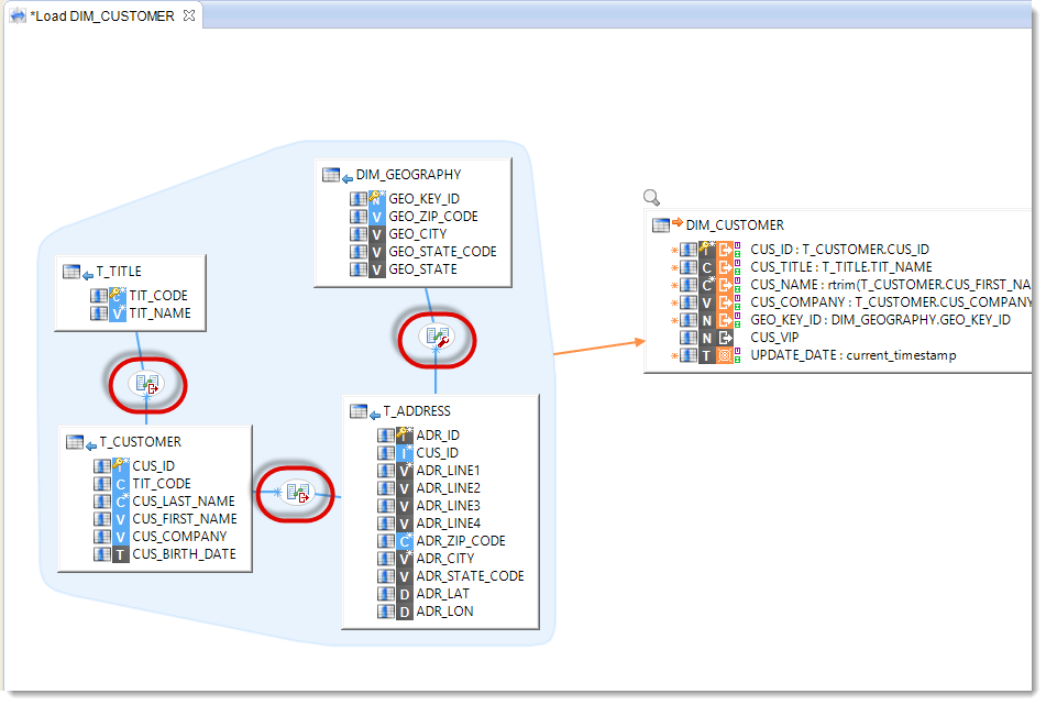
Creating the Mapping that loads the DIM_CUSTOMER table
Create a new Mapping with the following properties:
| Property | Value |
|---|---|
| Parent folder | Mappings |
| Mapping name | Load DIM_CUSTOMER |
| Target Datastore | DIM_CUSTOMER |
| Source Datastores | T_CUSTOMER, T_TITLE, T_ADDRESS, DIM_GEOGRAPHY |
The transformation business rules are:
| Target column | Business rule | Execution location | Activate |
|---|---|---|---|
| CUS_ID | T_CUSTOMER.CUS_ID |
Source | I/U |
| CUS_TITLE | T_TITLE.TIT_NAME |
Source | I/U |
| CUS_NAME | rtrim(T_CUSTOMER.CUS_FIRST_NAME) + ' ' + upper(rtrim(T_CUSTOMER.CUS_LAST_NAME)) |
Source | I/U |
| CUS_COMPANY | T_CUSTOMER.CUS_COMPANY |
Source | I/U |
| GEO_KEY_ID | DIM_GEOGRAPHY.GEO_KEY_ID |
Source | I/U |
| UPDATE_DATE | current_timestamp |
Target | I/U |
| CUS_VIP | (This column will be loaded further on in the tutorial) |
The join business rules are:
| First Datastore | Second Datastore | Business rule | Execution location |
|---|---|---|---|
| T_CUSTOMER | T_TITLE | T_CUSTOMER.TIT_CODE=T_TITLE.TIT_CODE |
Source |
| T_CUSTOMER | T_ADDRESS | T_CUSTOMER.CUS_ID=T_ADDRESS.CUS_ID |
Source |
| T_ADDRESS | DIM_GEOGRAPHY | DIM_GEOGRAPHY.GEO_ZIP_CODE=T_ADDRESS.ADR_ZIP_CODE |
Staging Area |
Important: Notice when you add the joins that the number of Load steps diminishes from 3 to 1. Indeed, Stambia Designer, thanks to its E-LT architecture, can optimize the Mappings by executing the business rules on the source as soon as possible. So the flow that is transferred between the source and target systems is reduced to the strict minimum.
Defining outer joins
One of the constraints of this Mapping is that you must fetch all the records that are in T_CUSTOMER. But joins can filter out elements. For example, let us imagine that a record of T_CUSTOMER has no matching address in T_ADDRESS, if nothing is done about it, this customer will not be charged because of the inner join (also called strict join because only data whose key exists in the two tables will be sent back by the request). So you must define an outer join, to make sure all the records of T_CUSTOMER are taken into account, even those that have no match in T_ADDRESS:
- Click on the join between T_CUSTOMER and T_ADDRESS
- Go to the Properties view
- Select the radio button next to T_CUSTOMER to define it as master table (main table) for the outer join.
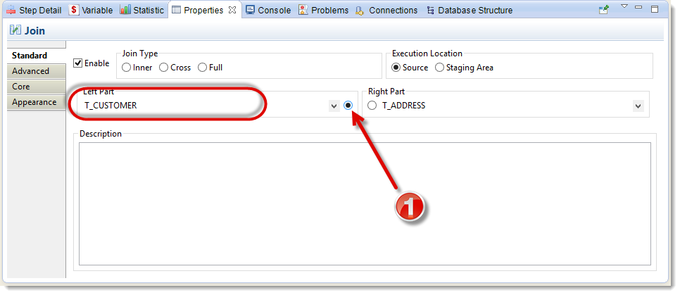
You can now notice that an icon in the form of an asterisk appears between the join icon and T_CUSTOMER. This is a visual aid for checking the side of the outer join.
![]()
Follow the same procedure to define the following outer joins:
| First Datastore | Second Datastore | Master table |
|---|---|---|
| T_CUSTOMER | T_ADDRESS | T_CUSTOMER |
| T_CUSTOMER | T_TITLE | T_CUSTOMER |
| T_ADDRESS | DIM_GEOGRAPHY | T_ADDRESS |
Visually, you should see all the asterisks of your Mapping on the side of T_CUSTOMER.
You can now execute the Mapping.
Analyzing the result of the execution
Go to the Statistic view to check the statistics of this execution:
| Name | Value |
|---|---|
SUM(SQL_NB_ROWS) |
300 |
SUM(SQL_STAT_INSERT) |
100 |
SUM(SQL_STAT_UPDATE) |
0 |
You can also check that the following request produces the value 11. Right-click on the target Datastore and select Action and Consult data then modify the request as follows:select count(*) from HOTEL_DATAMART.DIM_CUSTOMER where GEO_KEY_ID is null
When executing this request, you should see the value 11 show up on the result grid.
Indeed, the source data contains 11 customers that have no recorded address or with an incorrect address. The outer joins defined in this Mapping insert the customers, but with their addresses set to NULL.
Reject detection
What is reject detection?
In all data integration processes, one of the major issues is data quality. Of course, data have to be consistent with the technical expectations of the target database (foreign keys, unique keys, etc.), but they also have to be in accordance with the needs of the end users.
Stambia provides the ability to answer these two needs. On the one hand, reject detection mechanisms are a native part of the tool. On the other hand, you can enhance the metadata by adding extra user-defined constraints.
Finally, for each of these constraints, whether technical or functional, Stambia can:
- Detect the data that has to be rejected
- Set apart from the main dataflow the rejected data
Creating user-defined constraints on DIM_CUSTOMER
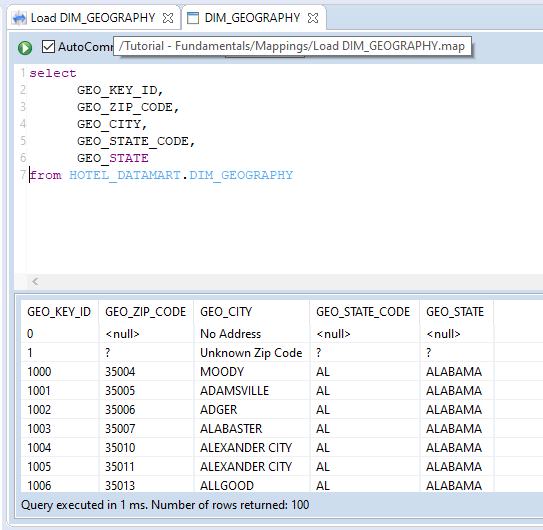
Particular values have been pre-recorded in the target database, in the DIM_GEOGRAPHY table:
| GEO_KEY_ID | GEO_ZIP_CODE | GEO_CITY | GEO_STATE_CODE | GEO_STATE |
|---|---|---|---|---|
0 |
<null> |
No Address |
<null> |
<null> |
1 |
? |
Unknown Zip Code |
? |
? |
Let’s assume that you want to track, on each integration, the data that are concerned by these special values. You will now create two constraints on DIM_CUSTOMER in order to check that the GEO_KEY_ID column in DIM_CUSTOMER does not contain the special values 0 or 1. Creating additional constraints is done in the Metadata file, by overloading the existing constraints:
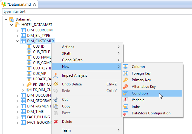
- Double-click on the Metadata file Datamart to open the Metadata editor.
- Find and unfold the DIM_CUSTOMER node
- Right-click on DIM_CUSTOMER
- Select New then
 Condition
 - Configure the Properties of the Condition
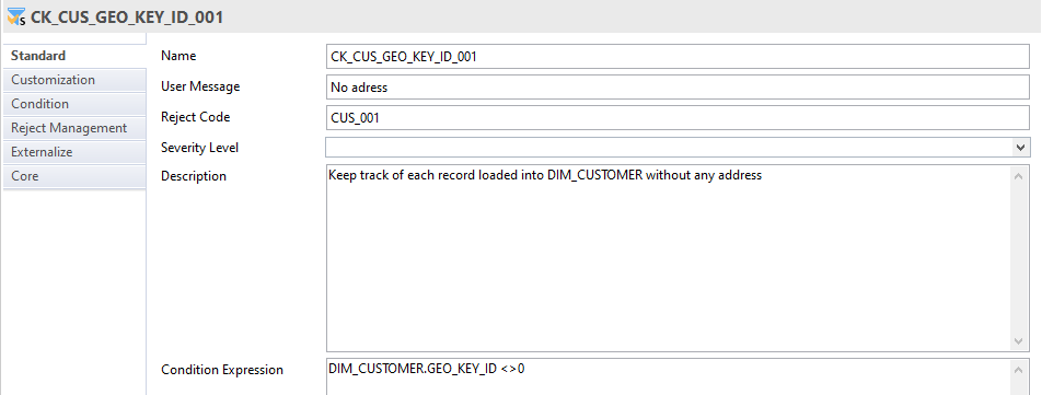
- In the Name field, enter a name for the new constraint: CK_CUS_GEO_KEY_ID_001
- In the Description field, you can freely document the new constraint: Keep track of each record loaded into DIM_CUSTOMER without any address
- In the Condition / Condition Expression field, enter the SQL code for the condition that the valid fields must verify:
DIM_CUSTOMER.GEO_KEY_ID <> 0 - The Reject Management / User Message field enables you to add a functional message to the reject: No address
- The Reject Management / Reject Code field enables you to add a technical identifier to the reject so that the reason for the rejection can be technically identified: CUS_001
Creating a new Condition
Defining Name and Description
Defining Reject Management information (User Message and Reject Code)
Defining Condition Expression
In the same way, create a second condition on DIM_CUSTOMER with the following properties:
| Property | Value |
|---|---|
| Name | CK_CUS_GEO_KEY_ID_002 |
| Description | Keep track of each record loaded into DIM_CUSTOMER with an address containing an unknown Zip Code |
| Condition Expression | DIM_CUSTOMER.GEO_KEY_ID <> 1 |
| User Message | Unknown Zip Code |
| Reject Code | CUS_002 |
Tip: To save time, you can copy the first condition you created, paste it in DIM_CUSTOMER and change the values.
Information: The reason for defining two different constraints is to gain more readability in the user messages. It would have been possible to create one global condition with the following Sql Condition:
DIM_CUSTOMER.GEO_KEY_ID not in (0,1).
Using default values in Load DIM_CUSTOMER
In order to make use of these new conditions, the first thing to do is to modify the business rule that loads DIM_CUSTOMER. Indeed, for the moment, because of the outer joins, this rule loads the GEO_KEY_ID field with the value found in DIM_GEOGRAPHY or with NULL if it is not to be found:
- Open the Mapping Load DIM_CUSTOMER
- Click on the target column GEO_KEY_ID
- In the Expression Editor view, replace the existing expression by the following:
case
when T_ADDRESS.ADR_ID is null then 0
when T_ADDRESS.ADR_ID is not null and DIM_GEOGRAPHY.GEO_KEY_ID is null then 1
else DIM_GEOGRAPHY.GEO_KEY_IDend
Information: Notice that Stambia Designer offers you some help to develop when you modify the business rule for the GEO_KEY_ID column: a red icon shows you that this rule is not correct because the default execution on the Source cannot be done since there are two different sources involved (if you leave your mouse pointer a few seconds on the red icon, a tooltip will appear).
Change the business rule so that it now executes in the Staging Area.
Implementing reject detection on Load DIM_CUSTOMER
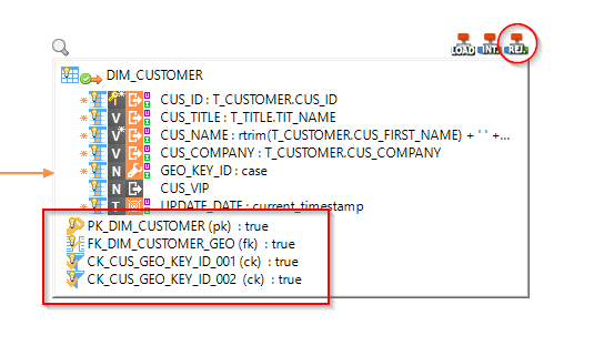
Everything is now ready for you to activate reject detection on the Mapping Load DIM_CUSTOMER:
- Select the DIM_CUSTOMER Datastore
- Click on the
 icon that appears to the left of the datastore to activate reject management.
Information: You can also activate reject management via the Properties view, once you have clicked on the target Datastore or right-clicked on it and selected Enable Rejects.
A new step will be added to the Mapping. It is the Check step to detect the rejects. Moreover, the DIM_CUSTOMER Datastore now displays the constraints that can be controlled.
In this Mapping, we want to keep track of the rejects without removing them from the dataflow. To do this:
- Click on the Check: DIM_CUSTOMER step (the «REJ» icon seen earlier)
- Open the Properties view
- Click on the link Delete Rejects On Checked Table in order to activate the box.
- Make sure this box is unchecked
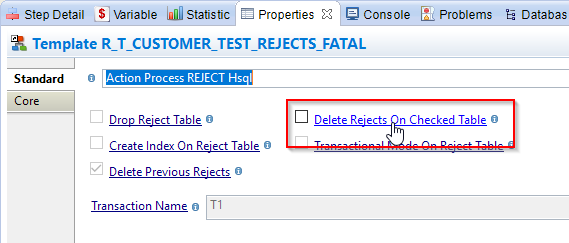
Your Mapping is now configured to detect rejects and keep track of them, without removing them from the dataflow. You can now execute the Mapping.
Analyzing the result of the execution
Go to the Statistic view to check the statistics of this execution:
| Name | Value |
|---|---|
SUM(SQL_NB_ROWS) |
322 |
SUM(SQL_STAT_ERROR) |
11 |
SUM(SQL_STAT_INSERT) |
0 |
SUM(SQL_STAT_UPDATE) |
11 |
Information: You can notice that a new statistic has appeared. It gives the number of rejects. Please check that there were 11 rejects detected.
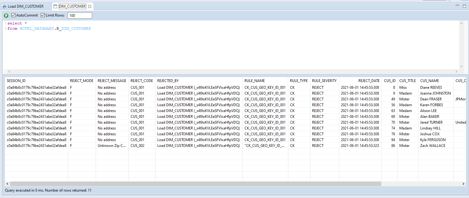
You can also consult the reject table to see what has been detected during the execution:
- Right-click on the target Datastore DIM_CUSTOMER
- Select Action then Consult Reject Table
- Execute the request
You can now see the 11 lines that were in error.
You can also check that the following request sends back a value of 10. Right-click on the target Datastore and select Action then Consult data and modify the request as follows:select count(*) from HOTEL_DATAMART.DIM_CUSTOMER where GEO_KEY_ID = 0
When executing this request, you should see 10 appear in the result grid.
In the same way, the following request should send back the value 1:select count(*) from HOTEL_DATAMART.DIM_CUSTOMER where GEO_KEY_ID = 1
Creating a Mapping with deduplicating
Creating the Mapping that loads DIM_TIME
Create a new Mapping with the following properties:
| Property | Value |
|---|---|
| Parent folder | Mappings |
| Mapping name | Load DIM_TIME |
| Target Datastore | DIM_TIME |
| Source Datastores | Time |
The transformation business rules are:
| Target column | Business rule | Characteristics | ||
|---|---|---|---|---|
| TIME_KEY_DAY | substr(Time.DAY_DATE, 7,4) + '/' + substr(Time.DAY_DATE, 4,2) + '/' + substr(Time.DAY_DATE, 1,2) |
Staging Area | I/U | Functional key |
| TIME_DATE | convert(substr(Time.DAY_DATE, 7,4) + '-' + substr(Time.DAY_DATE, 4,2) + '-' + substr(Time.DAY_DATE, 1,2) + ' 00:00:00',TIMESTAMP) |
Staging Area | I/U | |
| TIME_MONTH_DAY | convert(substr(Time.DAY_DATE, 1,2),NUMERIC) |
Staging Area | I/U | |
| TIME_WEEK_DAY | dayofweek(CONVERT(substr(Time.DAY_DATE, 7,4) + '-' + substr(Time.DAY_DATE, 4,2) + '-' + substr(Time.DAY_DATE, 1,2) + ' 00:00:00',TIMESTAMP)) |
Staging Area | I/U | |
| TIME_DAY_NAME | dayname(convert(substr(Time.DAY_DATE, 7,4) + '-' + substr(Time.DAY_DATE, 4,2) + '-' + substr(Time.DAY_DATE, 1,2) + ' 00:00:00', TIMESTAMP)) |
Staging Area | I/U | |
| TIME_MONTH | convert(substr(Time.DAY_DATE,4,2),NUMERIC) |
Staging Area | I/U | |
| TIME_MONTH_NAME | monthname(convert(substr(Time.DAY_DATE, 7,4) + '-' + substr(Time.DAY_DATE, 4,2) + '-' + substr(Time.DAY_DATE, 1,2) + ' 00:00:00',TIMESTAMP)) |
Staging Area | I/U | |
| TIME_QUARTER | quarter(convert(substr(Time.DAY_DATE, 7,4) + '-' + substr(Time.DAY_DATE, 4,2) + '-' + substr(Time.DAY_DATE, 1,2) + ' 00:00:00',TIMESTAMP)) |
Staging Area | I/U | |
| TIME_YEAR | convert(substr(Time.DAY_DATE, 7,4),NUMERIC) |
Staging Area | I/U | |
Tip: To define the execution location once for all the business rules, you can use multiselection by drawing a rectangle around the columns you wish to select. You can also do CTRL+click on each target column to refine the selection, or again select the first column, then keep the CAPS key pressed while clicking on the last column. Once the columns are selected, you can define the execution location (in this case Staging Area).
Implementing the deduplication
When consulting the data in the Time file, you may notice that there is one record for every 6 hour time slot. So for one day, there are 4 different lines:
01/01/2010 00:0001/01/2010 06:0001/01/2010 12:0001/01/2010 18:0002/01/2010 00:0002/01/2010 06:0002/01/2010 12:0002/01/2010 18:0003/01/2010 00:0003/01/2010 06:00
However, the DIM_TIME table expects only one line a day. So you must filter out the duplicates from the dataflow:
- Click on the Integration: DIM_TIME template
- Open the Properties view
- Click on the link Use distinct in order to activate the checking box.
- Make sure this box is checked
You have now configured the Template so that it eliminates duplicates.
You can now execute the Mapping.
Analyzing the result of the execution
Go to the Statistic view to check the statistics of the execution:
| Name | Value |
|---|---|
SUM(SQL_NB_ROWS) |
6 576 |
SUM(SQL_STAT_INSERT) |
1 096 |
SUM(SQL_STAT_UPDATE) |
0 |
Mutualizing transformations
Modifying the Mapping that loads DIM_TIME
When looking at the transformation rules hereabove, you will notice that they reuse many times the same expressions.
| Target column | Business rule | Characteristics | ||
|---|---|---|---|---|
| TIME_KEY_DAY | substr(Time.DAY_DATE, 7,4) + '/' + substr(Time.DAY_DATE, 4,2) + '/' + substr(Time.DAY_DATE, 1,2) |
Staging Area | I/U | Functional key |
| TIME_DATE | convert(substr(Time.DAY_DATE, 7,4) + '-' + substr(Time.DAY_DATE, 4,2) + '-' + substr(Time.DAY_DATE, 1,2) + ' 00:00:00',TIMESTAMP) |
Staging Area | I/U | |
| TIME_MONTH_DAY | convert(substr(Time.DAY_DATE, 1,2),NUMERIC) |
Staging Area | I/U | |
| TIME_WEEK_DAY | dayofweek(convert(substr(Time.DAY_DATE, 7,4) + '-' + substr(Time.DAY_DATE, 4,2) + '-' + substr(Time.DAY_DATE, 1,2) + ' 00:00:00',TIMESTAMP)) |
Staging Area | I/U | |
| TIME_DAY_NAME | dayname(convert(substr(Time.DAY_DATE, 7,4) + '-' + substr(Time.DAY_DATE, 4,2) + '-' + substr(Time.DAY_DATE, 1,2) + ' 00:00:00', TIMESTAMP)) |
Staging Area | I/U | |
| TIME_MONTH | convert(substr(Time.DAY_DATE,4,2),NUMERIC) |
Staging Area | I/U | |
| TIME_MONTH_NAME | monthname(convert(substr(Time.DAY_DATE, 7,4) + '-' + substr(Time.DAY_DATE, 4,2) + '-' + substr(Time.DAY_DATE, 1,2) + ' 00:00:00',TIMESTAMP)) |
Staging Area | I/U | |
| TIME_QUARTER | quarter(convert(substr(Time.DAY_DATE, 7,4) + '-' + substr(Time.DAY_DATE, 4,2) + '-' + substr(Time.DAY_DATE, 1,2) + ' 00:00:00',TIMESTAMP)) |
Staging Area | I/U | |
| TIME_YEAR | convert(substr(Time.DAY_DATE, 7,4),NUMERIC) |
Staging Area | I/U | |
Stambia Designer enables to mutualize these expressions with the help of a Stage, then to reuse them when loading a datastore.
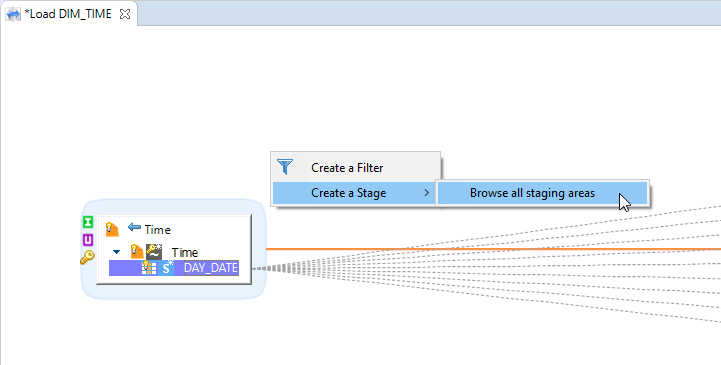
To create a Stage, drag-and-drop the DAY_DATE column on the Mapping.
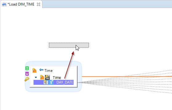
Select Create a Stage > Browse all staging areas
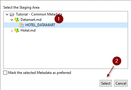
A dialog box will open to choose a schema on which to create the Stage
Select HOTEL_DATAMART schema
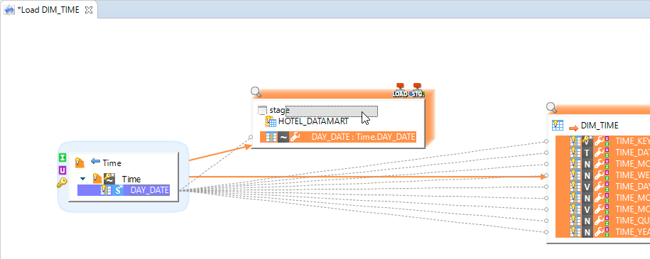
You can now rename this Stage to give it a more convenient name:
- For this select the Stage
- In the Properties view, enter mutualization in the Alias field
Note that you can also create a Stage by drag-and-dropping the schema directly from Project Explorer View inside the Mapping.
You can now add and define all the necessary fields for mutualizing transformations.
Expressions for Stage fields are defined as you would do for a target column.
To create a new field on an existing Stage, you can drag-and-drop a column on the Stage
Note that you can also click on the  icon to create an empty field.
To change the name of a field, select it, and then change its Alias in the Properties view.
Complete this Stage with the following columns:
| Target column | Business rule |
|---|---|
| DAY_DATE | convert(substr(Time.DAY_DATE, 7,4) + '-' + substr(Time.DAY_DATE, 4,2) + '-' + substr(Time.DAY_DATE, 1,2) + ' 00:00:00',TIMESTAMP) |
| TIME_MONTH_DAY | substr(Time.DAY_DATE, 1,2) |
| TIME_MONTH | substr(Time.DAY_DATE,4,2) |
| TIME_YEAR | substr(Time.DAY_DATE, 7,4) |
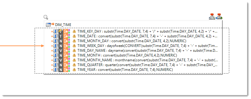
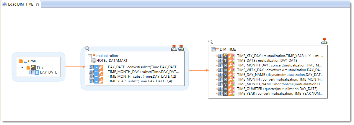
Now modify the business rules that load DIM_TIME in order to use the Stage columns:
| Target column | Business rule | Characteristics | ||
|---|---|---|---|---|
| TIME_KEY_DAY | mutualization.TIME_YEAR + '/' + mutualization.TIME_MONTH + '/' + mutualization.TIME_MONTH_DAY |
Staging Area | I/U | Functional key |
| TIME_DATE | mutualization.DAY_DATE |
Staging Area | I/U | |
| TIME_MONTH_DAY | convert(mutualization.TIME_MONTH_DAY,NUMERIC) |
Staging Area | I/U | |
| TIME_WEEK_DAY | dayofweek(mutualization.DAY_DATE) |
Staging Area | I/U | |
| TIME_DAY_NAME | dayname(mutualization.DAY_DATE) |
Staging Area | I/U | |
| TIME_MONTH | convert(mutualization.TIME_MONTH,NUMERIC) |
Staging Area | I/U | |
| TIME_MONTH_NAME | monthname(mutualization.DAY_DATE) |
Staging Area | I/U | |
| TIME_QUARTER | quarter(mutualization.DAY_DATE) |
Staging Area | I/U | |
| TIME_YEAR | convert(mutualization.TIME_YEAR,NUMERIC) |
Staging Area | I/U | |
You can now execute the Mapping.
Analyzing the result of the execution
Go to the Statistic view to check the statistics of the execution:
| Name | Value |
|---|---|
SUM(SQL_NB_ROWS) |
6 576 |
SUM(SQL_STAT_INSERT) |
0 |
SUM(SQL_STAT_UPDATE) |
0 |
You can see that mutualizing the transformations did not change the table contents (no insert and no update were executed on DIM_TIME) and that the results are indeed the same.
Loading a datastore through the union of various sources
Modifying the Mapping that loads DIM_TIME
The DIM_TIME datastore must be loaded from the Time.csv file on the one hand and from the T_PLANNING table on the other hand. Instead of creating two load mappings for the same table, Stambia Designer enables to realize a union of the data from these two sources before integrating them into the target.
Creation of this dataset takes place on the Stage meant to make the union of the data:
- Select the mutualization Stage
- Click on the
 icon to the left of the Stage
The Stage then displays both datasets A and B.
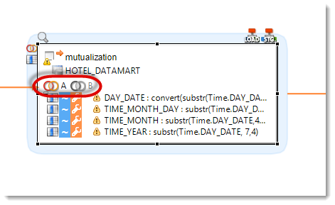
To facilitate reading, rename each dataset:
- Select the dataset A
- In the Properties view, enter File in the Alias field
In the same way, rename the dataset B into Rdbms.
Now specify the type of union between these datasets:
- Select the mutualization Stage
- In the Expression Editor enter the business rule:
[File] union [Rdbms]
This new set will be loaded from the T_PLANNING table which includes other dates than the Time.csv file. Begin by adding the T_PLANNING Datastore to the Mapping. Then, to specify the business rules for this second dataset, select the Rdbms set and enter the following business rules:
| Target column | Business rule |
|---|---|
| DAY_DATE | T_PLANNING.PLN_DAY |
| TIME_MONTH_DAY | lpad(day(T_PLANNING.PLN_DAY), 2, '0') |
| TIME_MONTH | lpad(month(T_PLANNING.PLN_DAY), 2, '0') |
| TIME_YEAR | convert(year(T_PLANNING.PLN_DAY), VARCHAR) |
You can now execute the Mapping.
Analyzing the result of the execution
Go to the Statistic view to check the statistics of the execution:
| Name | Value |
|---|---|
SUM(SQL_NB_ROWS) |
9 132 |
SUM(SQL_STAT_INSERT) |
730 |
SUM(SQL_STAT_UPDATE) |
0 |
Exercise: Creating a Simple Mapping
Creating the Mapping that loads FACT_BOOKING
Create and execute the following Mapping:
| Property | Value |
|---|---|
| Parent folder | Mappings |
| Mapping name | Load FACT_BOOKING |
| Target Datastore | FACT_BOOKING |
| Source Datastores | DIM_TIME, T_BDR_PLN_CUS |
The transformation business rules are:
| Target column | Business rule | Characteristics | ||
|---|---|---|---|---|
| BOK_KEY_ID | ||||
| CUS_ID | T_BDR_PLN_CUS.CUS_ID |
Source | I/U | Functional key |
| TIME_KEY_DAY | DIM_TIME.TIME_KEY_DAY |
Source | I/U | Functional key |
| BDR_ID | T_BDR_PLN_CUS.BDR_ID |
Source | I/U | Functional key |
| BOK_PEOPLE | T_BDR_PLN_CUS.PLN_CUS_PERS_COUNT |
Source | I/U | |
| BOK_BOOKED | casewhen T_BDR_PLN_CUS.PLN_CUS_BOOKED = 'true' then 1else 0end |
Source | I/U | |
| UPDATE_DATE | current_timestamp |
Target | I/U | |
Information: The BOK_KEY_ID column is an «auto-incremented» field, which means it is created in the database so as to create an identifier for every insertion. This is why it must not be mapped, so that the database can load it itself.
The join business rules are:
| First Datastore | Second Datastore | Business rule | Execution Location |
|---|---|---|---|
| DIM_TIME | T_BDR_PLN_CUS | T_BDR_PLN_CUS.PLN_DAY=DIM_TIME.TIME_DATE |
Staging Area |
Analyzing the result of the execution
Go to the Statistic view to check the statistics of the execution:
| Name | Value |
|---|---|
SUM(SQL_NB_ROWS) |
43 650 |
SUM(SQL_STAT_INSERT) |
14 550 |
SUM(SQL_STAT_UPDATE) |
0 |
Creating a Mapping with aggregate calculation
Creating the Mapping that loads FACT_BILLING
Create the following Mapping:
| Property | Value |
|---|---|
| Parent folder | Mappings |
| Mapping name | Load FACT_BILLING |
| Target Datastore | FACT_BILLING |
| Source Datastores | T_BILLING, T_BILLING_LINES, DIM_TIME, DIM_DISCOUNT |
The transformation business rules are:
| Target column | Business rule | Characteristics | ||
|---|---|---|---|---|
| BIL_KEY_ID | ||||
| BIL_ID | T_BILLING.BIL_ID |
Source | I/U | Functional key |
| CUS_ID | T_BILLING.CUS_ID |
Source | I/U | |
| TIME_KEY_DAY | DIM_TIME.TIME_KEY_DAY |
Source | I/U | |
| DIS_RANGE | DIM_DISCOUNT.DIS_RANGE |
Source | I/U | Functional key |
| PMT_CODE | T_BILLING.PMT_CODE |
Source | I/U | |
| BIL_AMOUNT | sum(T_BILLING_LINES.BLL_AMOUNT) |
Staging Area | I/U | |
| BIL_QTY | sum(T_BILLING_LINES.BLL_QTY) |
Staging Area | I/U | |
| UPDATE_DATE | current_timestamp |
Target | I/U | |
The join business rules are:
| First Datastore | Second Datastore | Business rule | Execution location |
|---|---|---|---|
| T_BILLING | DIM_TIME | T_BILLING.BIL_DATE=DIM_TIME.TIME_DATE |
Staging Area |
| T_BILLING | T_BILLING_LINES | T_BILLING_LINES.BIL_ID=T_BILLING.BIL_ID |
Source |
| T_BILLING_LINES | DIM_DISCOUNT | round(casewhen T_BILLING_LINES.BLL_DISCOUNT_AMOUNT != 0then (T_BILLING_LINES.BLL_DISCOUNT_AMOUNT / (T_BILLING_LINES.BLL_AMOUNT + T_BILLING_LINES.BLL_DISCOUNT_AMOUNT))*100else T_BILLING_LINES.BLL_DISCOUNT_RATEend)between DIM_DISCOUNT.DIS_MIN and DIM_DISCOUNT.DIS_MAX |
Staging Area |
Before you can execute the Mapping, you must tell Stambia Designer which are the columns for which the business rules are aggregations:
- Select the target column BIL_AMOUNT
- Click on the
 icon to the left of the Datastore to activate aggregation of this column.
Do the same for the BIL_QTY column.
You can now execute the Mapping.
Analyzing the result of the execution
Go to the Statistic view to check the statistics of the execution:
| Name | Value |
|---|---|
SUM(SQL_NB_ROWS) |
53 314 |
SUM(SQL_STAT_INSERT) |
12 107 |
SUM(SQL_STAT_UPDATE) |
0 |
Adding an extra constraint
Exercise text
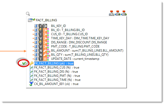
Create a new constraint on FACT_BILLING which will check that the value of the BIL_AMOUNT column contains values greater than 10:FACT_BILLING.BIL_AMOUNT > 10
Then check this new constraint by activating the reject detection in the Load FACT_BILLING Mapping. The purpose is not to remove the data from the flow, but simply to keep track of them in the Reject table.
Tip: If you are not sure of the procedure, you can go and look at Implementing reject detection on Load DIM_CUSTOMER
Warning: The BIL_KEY_ID column is not loaded by this Mapping but auto-loaded by the database. This means you will not be able to check the primary key of FACT_BILLING, during the reject detection step. To disable this control, select PK_FACT_BILLING (pk) : true then click on the
Analyzing the result of the execution
After having executed the mapping once it has been modified to take into account reject detection, go to the Statistic view to check the statistics of the execution:
| Name | Value |
|---|---|
SUM(SQL_NB_ROWS) |
53 316 |
SUM(SQL_STAT_ERROR) |
2 |
SUM(SQL_STAT_INSERT) |
0 |
SUM(SQL_STAT_UPDATE) |
0 |
You can also check in the Reject table that 2 lines (numbers 224 and 5994 of BIL_ID) have been tracked down.
Automating the loading of the Datamart
Presentation of the Processes
A Process is a set of Actions executed by the Runtime. For each execution of the Mappings you did earlier, Stambia generated a Process from each Mapping. This is the Process you were able to consult at each execution of a Mapping.
However, you can also create Processes manually to orchestrate higher level components (Mappings or even other Processes) as well as unit action of a lower level (SQL commands, file handling and a lot of other tools are available).
Creating a general orchestration Process
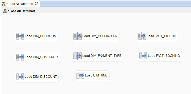
Creating the Process that loads all the Datamart
Create a Process which will execute all the loading of the Datamart:
- Unfold the Project Tutorial – Fundamentals
- Right-click on the folder Processes
- Select New then Process
- In the File name field, enter the value: Load All Datamart
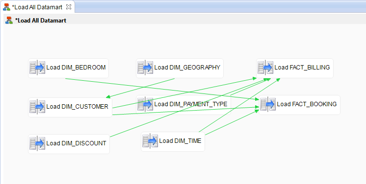
Adding the Mappings
Add each of the Mappings you developed previously:
- In the Project Explorer view, select a Mapping
- Drag and drop this Mapping into the Process editor
Defining the links
By default, Stambia executes each step of a Process concurrently from the beginning of the Process. However, because of the foreign keys that are in the target model, you need to set an order for the execution of certain mappings. To do this, you will create a link between these Mappings:
- Select the origin step.
- Select the green arrow and drag it to the end step.
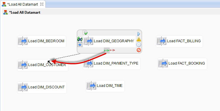
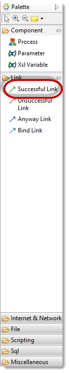
Alternatively you can use the Palette to define a link:
- In the Palette of components, unfold the Link drawer
- Select the component
 Successful Link
 - Now draw an arrow between the Mappings you have to link: drag and drop from the Mapping which must execute first towards the Mapping which must execute after.
In order for the Process to execute properly, you will link the steps in the following way:
| Origin step | End step |
|---|---|
| DIM_GEOGRAPHY | DIM_CUSTOMER |
| DIM_CUSTOMER | FACT_BOOKING |
| DIM_TIME | FACT_BOOKING |
| DIM_BEDROOM | FACT_BOOKING |
| DIM_CUSTOMER | FACT_BILLING |
| DIM_TIME | FACT_BILLING |
| DIM_DISCOUNT | FACT_BILLING |
| DIM_PAYMENT_TYPE | FACT_BILLING |
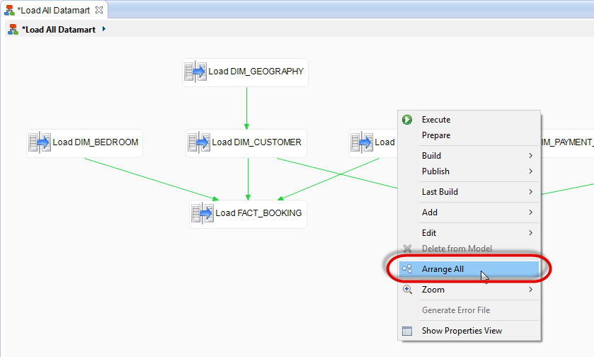
Finally, to increase the readability of your diagram, you can use the automatic reorganization function:
- Right-click on the background of the Process diagram
- Select Arrange All
Executing the Process
You can now execute the Process:
- Right-click on the background of the Process diagram
- Select Execute
Analyzing the result of the execution
Go to the Statistic view to check the statistics of the execution:
| Name | Value |
|---|---|
SUM(SQL_NB_ROWS) |
232 140 |
SUM(SQL_STAT_ERROR) |
13 |
SUM(SQL_STAT_INSERT) |
0 |
SUM(SQL_STAT_UPDATE) |
0 |
Adding empty steps
In order to further increase a diagram’s readability, or to facilitate the ordering of many parallel tasks, it is sometimes useful to add empty steps so as to define specific synchronization points.
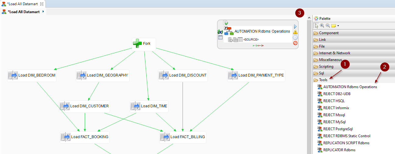
Further on, you will be adding steps to this Process before the first step and after the last step of the loading procedure. To make this easier, you will add an empty step at the beginning of the Process:
- In the Palette of components, unfold the Miscellaneous drawer
- Select the component
 Empty action
 - Click inside the diagram to create the empty step
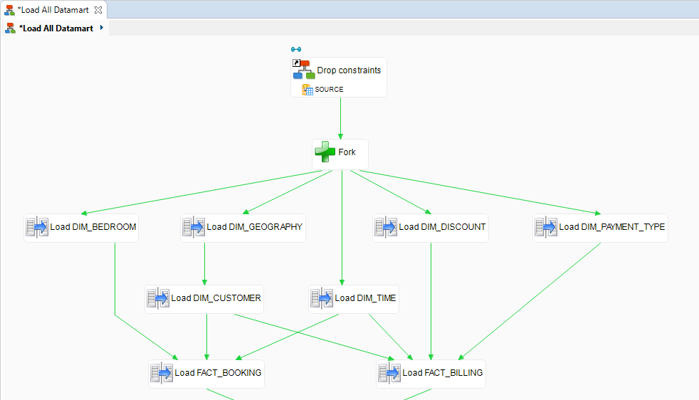
- Type the name of this action: Fork
![]()
You can now link this step to the first steps of the loading procedure:
| Origin step | End step |
|---|---|
| Fork | DIM_GEOGRAPHY |
| Fork | DIM_TIME |
| Fork | DIM_BEDROOM |
| Fork | DIM_DISCOUNT |
| Fork | DIM_PAYMENT_TYPE |
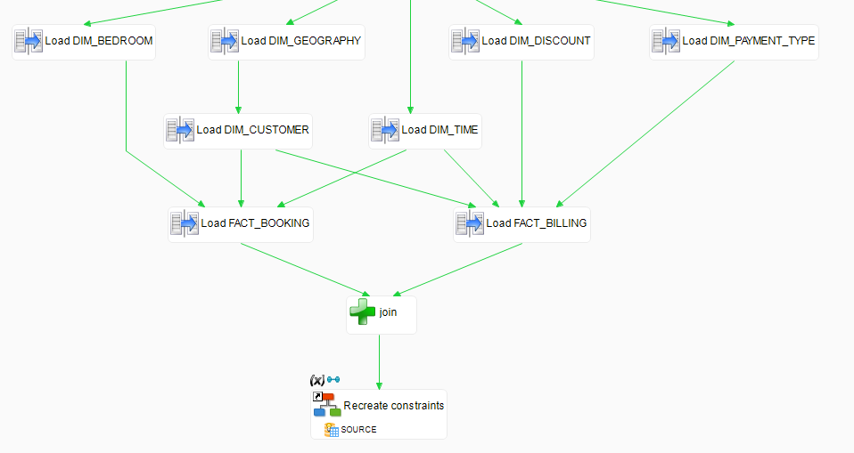
In the same way, create an empty step called Join to terminate the loading procedure.
![]()
Allowing disabling/enabling of the constraints
Adding a step that disables all the schema’s constraints
The Stambia Templates allow you to automatize actions on metadata to automatically generate Processes and thus industrialize the developments. For example, a template can iterate on the table list of a database schema to carry out an operation.
For example, you can take advantage of this functionality to disable constraints at the beginning of the loading procedure and recreate them at the end. This means the underlying database will not check the constraints during the loading procedure and the performances will be enhanced.
To create a step that disables constraints:
- Unfold the global project in the Project Explorer view
- Then unfold the template.generic node then Automation
- Drag and drop the AUTOMATION Rdbms Operations.tp template on the Process diagram
Now configure this new step:
- Click on the step newly created and open the Properties view
- In the Name field, enter the value Drop constraints
- Click on the link Drop Fk and check that the checkbox is checked
Next, this template needs to know the schema with all the tables it has to affect:
- Unfold the node of the Metadata file Datamart then the one of the Datamart server
- Drag and drop the schema HOTEL_DATAMART onto the header (title) of the step Drop constraints
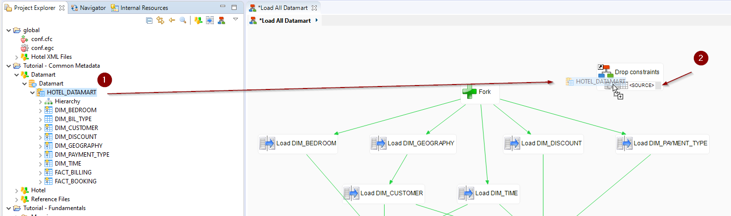
Finally, you have to link this step to the current starting step Fork.
Adding a step that reactivates all the constraints of the schema
Proceed in the same way to create a step which will recreate all the constraints of the schema. Of course, you will choose the option Create Fk instead of Drop Fk you previously used.
Name this step Recreate constraints.
You can now execute the Process.
Analyzing the result of the execution
Go to the Statistic view to check the statistics of this execution:
| Name | Value |
|---|---|
SUM(SQL_NB_ROWS) |
232 140 |
SUM(SQL_STAT_ERROR) |
13 |
SUM(SQL_STAT_INSERT) |
0 |
SUM(SQL_STAT_UPDATE) |
0 |
You can then check the generated code by opening for example the Drop constraints step then Drop FK.
The under-process that opens is composed of one single under-process Fk for table which was instantiated 3 times. Indeed, this under-process is configured to be executed for every table that has a foreign key. This is why the name that is given is Fk for table 3/3.
With this kind of step, you need to select the right instantiation:
- Select the under-process Fk for table 3/3
- Open the Step Detail view
- In the Detail of drop-down list, you can choose the instantiation of this under-process you wish to consult
- Select Fk for table – FACT_BILLING
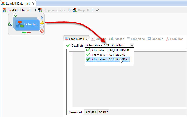
You can now double-click on Fk for table 3/3 to open this instantiation of the under-process.
The FACT_BILLING table has 4 foreign keys. This is why the name of the action is Drop FK 4/4.
Follow the same technique to look at the executed code for each of the foreign keys.
Adding default values
Adding a data purge
The next step in this Process is to purge all the data of all the tables, and reset the initial data (because some tables of the HOTEL_DATAMART base had lines that will have been removed by the automatic purge).
In order to purge the data from the tables, edit the step Drop constraints and select the Template option Delete Tables in addition to Drop Fk. With this new option, Stambia will purge all the data in the target tables.
Initializing the tables
There only remains to create actions that will insert again the data that are missing from the database:
- In the Palette of components, unfold the Sql drawer
- Select the component
 Sql Operation
 - Click inside the diagram to create an empty step
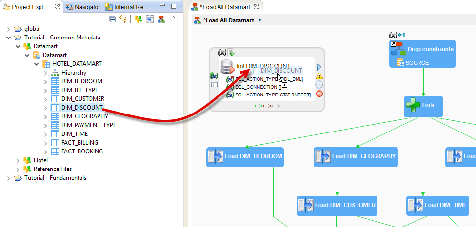
- Enter the name of this action: Init DIM_DISCOUNT
- In the Properties view, click on the link Sql Action Type Stat then enter the value
INSERT. - In the Expression Editor view enter the SQL command that is to be executed:
insert into HOTEL_DATAMART.DIM_DISCOUNT (DIS_RANGE, DIS_MIN, DIS_MAX) values ('No discount',NULL,NULL);
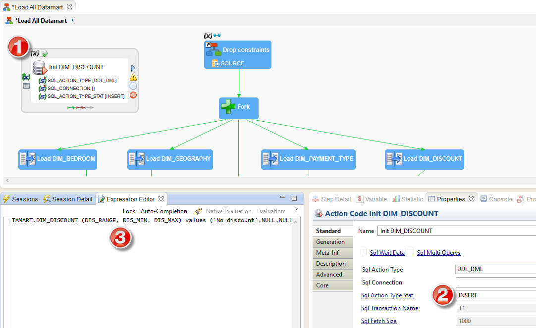
Finally, so that Stambia knows on which JDBC connection it has to execute this SQL command, you need to use a metadata link. Drag and drop the DIM_DISCOUNT Datastore onto this new step in order to create the metadata link.
Information: If you parameter the hereabove Sql Action Type Stat option, Stambia can count the number of inserted lines and integrate them to the Session statistics for the
INSERT(statistic SQL_STAT_INSERT).
Create a second SQL action with the following properties:
| Property | Value |
|---|---|
| Name | Init DIM_GEOGRAPHY |
| SQL code to execute | insert into HOTEL_DATAMART.DIM_GEOGRAPHY (GEO_KEY_ID, GEO_ZIP_CODE, GEO_CITY, GEO_STATE_CODE, GEO_STATE) values (0, NULL, 'No Address', NULL, NULL);insert into HOTEL_DATAMART.DIM_GEOGRAPHY (GEO_KEY_ID, GEO_ZIP_CODE, GEO_CITY, GEO_STATE_CODE, GEO_STATE) values (1, '?', 'Unknown Zip Code', '?', '?'); |
| Sql Action Type Stat | INSERT |
| Sql Multi Queries | <true> |
Important: Stambia allows the execution of several SQL commands in the same action if you use the parameter Sql Multi Queries. This parameter is used together with the Sql Multi Queries Separator parameter which defines the character that separates the various SQL orders (by default the semi-colon). The SQL orders statistics will be consolidated for all the SQL orders executed in the step.
Finally, link these two actions so that they execute concurrently between Drop constraints and Fork.
You can cow execute the Process.
Analyzing the result of the execution
Go to the Statistic view to check the statistics of the execution:
| Name | Value |
|---|---|
SUM(SQL_NB_ROWS) |
302 452 |
SUM(SQL_STAT_DELETE) |
70 309 |
SUM(SQL_STAT_ERROR) |
13 |
SUM(SQL_STAT_INSERT) |
70 309 |
SUM(SQL_STAT_UPDATE) |
0 |
Creating a report file
How to use the session variables?
When executing a session, Stambia deals with a lot of information:
- Execution duration of each step
- Temporary folder of the Runtime
- Hostname and port of the Runtime
- Session name
- Name of each step
- etc.
All this information is available in the form of Session Variables:
- Some of these variables can be directly accessed at the session level because they are global to the session. You can see them in the Session Detail view under the Variables tab.
- The other variables are dynamically created and given a value at each step of a process, and can be consulted in the Variables view. The Variables of the object selected inside the Process will be shown in this view.
The complete name of a variable depends on its location. To refer to a variable, you need to give its path:/VAR indicates a global Session Variable (the «/» represents the root of the session)
For a variable that is local to a step, you need to give its path right till this step, then the name of the variable:../Step/VAR indicates a variable that will be searched first in the father step of the current step, then in the current step called Step.
At any moment of the execution of the session, you can fetch the value of a variable with the following syntax:
${Variable}$
The value of the variable will then be substituted in the text. Please refer to the help section of Stambia, in the part about processes. The call syntax is detailed there.
Examples:
| Variable | Value |
|---|---|
${/CORE_DURATION}$ |
Execution duration of the session |
${../Init/CORE_DURATION}$ |
Execution duration of the Init step |
${../Init/First Value/CORE_DURATION}$ |
Execution duration of the First Value action which is in the Init step |
Creating the file containing the report of the execution
Create a step that allows you to write freely in a file:
- In the Palette of components, unfold the File drawer
- Select the component
 Write a File
 - Enter the name of this action: Write Execution Report
- In the Properties view, give the following value to the Txt Write Filename property:
${/CORE_TEMPORARY_FOLDER}$/Load_All_Datamart_Report.txt
This tells Stambia to write text in a file located in ${/CORE_TEMPORARY_FOLDER}$/Load_All_Datamart_Report.txt. The path of this location uses the session variable CORE_TEMPORARY_FOLDER which holds the path of the Runtime’s temporary folder (choose a session, and look in the Session Detail view, under the Variables tab to find the default value for your runtime).
Next, tell Stambia what text to write inside this file:
- Open the Expression Editor view
- Enter the following text:
Session started on: ${/CORE_BEGIN_DATE}$
Steps duration:
Load FACT_BILLING: ${../Load FACT_BILLING/CORE_DURATION}$
Load FACT_BOOKING: ${../Load FACT_BOOKING/CORE_DURATION}$
Recreate Fk : ${../Recreate constraints/Create FK/CORE_DURATION}$
Link this step so that it gets executed after recreating the constraints, then execute the Process.
Analyzing the result of the execution
Go to the Statistic view to check the statistics of the execution:
| Name | Value |
|---|---|
SUM(SQL_NB_ROWS) |
302 452 |
SUM(SQL_STAT_DELETE) |
70 309 |
SUM(SQL_STAT_ERROR) |
13 |
SUM(SQL_STAT_INSERT) |
70 309 |
SUM(SQL_STAT_UPDATE) |
0 |
Look at the code executed by the step Write Execution Report. You will notice that to see the text with the values of the variables, you have to click on the Executed tab in the Step Detail view.
Also, you can find the file Load_All_Datamart_Report.txt in the directory of your installation, in the folder stambiaRuntime then in temp.
Using scripting
Presentation of scripting in Stambia
Stambia allows you to interact with the Runtime in the course of a session, using a scripting language.
The general syntax to invoke scripting in Stambia is:
%e(language){ .... SCRIPT .... }e(language)%
The scripting languages available in Stambia are:
groovyjython(Python type syntax)rhino(JavaScript type syntax)
Moreover, Stambia provides an API which allows you to directly interact with the Runtime. This API __ctx__ can be used with any of these languages (it is a Java class with methods that are predefined and made available to the developer).
Information: For further information on scripting with Stambia please refer to the user’s guide of Stambia Designer.
Fetching the statistics in the report file
__ctx__.sumVariable() is one of the functions of Stambia which allows you to add up numerical variables of the Runtime:
__ctx__.sumVariable(<VAR>): sends back the sum of the values of the variable VAR for the whole Session.__ctx__.sumVariable(<VAR>, <STEP>): sends back the sum of the values of the variable VAR only for step STEP.
Information: There are other functions that are explained in the help section of Stambia.
Modify the Write Execution Report step in order to add the statistics for certain steps of the Process:
Total Rows: %e(rhino){__ctx__.sumVariable("SQL_NB_ROWS")}e(rhino)%Total Inserts: %e(rhino){__ctx__.sumVariable("SQL_STAT_INSERT")}e(rhino)%Inserts into FACT_BILLING: %e(rhino){__ctx__.sumVariable("SQL_STAT_INSERT","../Load FACT_BILLING")}e(rhino)%
Additional exercises
Enhancing the data of a table
In this exercise, you will have to update the existing records of the DIM_CUSTOMER table by giving values to the CUS_VIP column without touching the values that already exist. Here, we wish to find the VIP customers, which are the customers who have spent more than 64000$ since the hotel’s creation.
Creating the Mapping that enhances the DIM_CUSTOMER table
Create the following Mapping:
| Property | Value |
|---|---|
| Parent folder | Mappings |
| Mapping name | Load DIM_CUSTOMER.CUS_VIP (1) |
| Target Datastore | DIM_CUSTOMER |
| Source Datastores | T_BILLING, T_BILLING_LINES |
The transformation business rules are:
| Target column | Business rule | Characteristics | ||
|---|---|---|---|---|
| CUS_ID | T_BILLING.CUS_ID |
Source | I/U | Functional key |
| CUS_TITLE | ||||
| CUS_NAME | ||||
| CUS_COMPANY | ||||
| GEO_KEY_ID | ||||
| UPDATE_DATE | current_timestamp |
Target | U | |
| CUS_VIP | casewhen sum(T_BILLING_LINES.BLL_QTY*((T_BILLING_LINES.BLL_AMOUNT-T_BILLING_LINES.BLL_DISCOUNT_AMOUNT) - (T_BILLING_LINES.BLL_AMOUNT * T_BILLING_LINES.BLL_DISCOUNT_RATE / 100))) > 64000 then 1else 0end |
Source, Aggregate | U | |
Information: Notice that the Mapping of the CUS_VIP column is only enabled for Updates and especially that the other target columns are not mapped. This means they will not be impacted by this Mapping’s execution.
The join business rules are:
| First Datastore | Second Datastore | Business rule | Execution location |
|---|---|---|---|
| T_BILLING | T_BILLING_LINES | T_BILLING_LINES.BIL_ID=T_BILLING.BIL_ID |
Source |
Analyzing the result of the execution
Go to the Statistic view to check the statistics of the execution:
| Name | Value |
|---|---|
SUM(SQL_NB_ROWS) |
400 |
SUM(SQL_STAT_INSERT) |
0 |
SUM(SQL_STAT_UPDATE) |
100 |
Then check that the data of the DIM_CUSTOMER table match the following information:
- There are 95 customers that are not VIP:
select count(*) from HOTEL_DATAMART.DIM_CUSTOMER where CUS_VIP != 1 - VIP customers have the following
CUS_ID: 7, 18, 75, 92 and 96:select CUS_ID from HOTEL_DATAMART.DIM_CUSTOMER where CUS_VIP = 1
Partial enhancing of a table
Creating the second Mapping that enhances the DIM_CUSTOMER table
In this exercise, you are going to update the CUS_VIP field with the following rules:
- If a customer was already identified as VIP, he must stay VIP
- If a customer has been billed for more than 30 stays in a
'suite'type room, he becomes a VIP. This means we have to check the records ofT_BILLING_LINES, as well as theDIM_BEDROOM.BDR_TYPEcolumn. - The column
UPDATE_DATEmust be set with the current date and time each time a record is updated.
Checking the result of the execution
Since there are many ways to solve this exercise, that will generate different statistics, you can check the content of the DIM_CUSTOMER table:
- There are 92 customers that are not VIP:
select count(*) from HOTEL_DATAMART.DIM_CUSTOMER where CUS_VIP != 1 - VIP customers have the following
CUS_ID: 7, 18, 31, 53, 75, 89, 92 et 96:select CUS_ID from HOTEL_DATAMART.DIM_CUSTOMER where CUS_VIP = 1
Information: If the result of the execution is wrong, you will have to come back to the initial state before you redo the exercise: execute the Load All Datamart Process, then execute the Load DIM_CUSTOMER.CUS_VIP (1) Mapping.
Frequent mistakes
Here are the most frequent mistakes that are encountered during this exercise.
How to select the customers who have been billed for more than 30 stays in a suite?
The easiest way to select these customers is to create a Filter in the mapping:
count(T_BILLING_LINES.BLL_ID) > 30
SQL Error: Not a condition
The SQL function count() is an aggregation function. So, when you create the filter, you need to tell Stambia Designer that this filter uses an aggregation function:
- Right-click on the
count(T_BILLING_LINES.BLL_ID) > 30filter - Select Aggregate
No VIP customer detected
This usually happens when the count(T_BILLING_LINES.BLL_ID) > 30 filter is executed on the Source.
Indeed, Stambia enables you to choose between 3 different locations to execute the expression: the source, the staging area and the target. For example, for the loading of DIM_BEDROOM, you executed the expression on the target for the column containing the timestamp. This concerns expressions that will be evaluated at the last moment, i.e. the moment when the data are integrated into the target table. Another location where Stambia can evaluate expressions is the staging area.
The staging area is the place where all source data are centralized in order to prepare them before they are integrated into the target.
Let’s use the following simplified data to give an example:
| BDR_ID | BDR_TYPE |
|---|---|
| 1 | suite |
| 2 | suite |
| 3 | suite |
| 4 | standard |
| 5 | standard |
| BLL_ID | CUS_ID | BDR_ID |
|---|---|---|
| 1 | 1 | 1 |
| 2 | 1 | 2 |
| 3 | 1 | 3 |
| 4 | 1 | 4 |
| 5 | 1 | 5 |
| 6 | 2 | 1 |
| 7 | 2 | 1 |
| 8 | 2 | 1 |
| 9 | 2 | 1 |
| 10 | 3 | 5 |
| 11 | 3 | 5 |
| 12 | 3 | 5 |
| 13 | 3 | 5 |
And let’s use the following filter: count(T_BILLING_LINES.BLL_ID) > 2
If we look at the data, we can see that customer CUS_ID=1 will be selected since he stayed in the rooms 1, 2 and 3 which are suites. Customer CUS_ID=2 will also be selected since he stayed 4 times in room 1 which is a suite.
If this filter is executed on the source, since Stambia needs the BDR_ID to do the join in the staging area, the request that will be executed on the source will be:
select BDR_ID, CUS_ID from T_BILLING_LINES group by BDR_ID, CUS_ID having count(BLL_ID) > 2
The resulting data will then be:
| CUS_ID | BDR_ID | count(BLL_ID) |
|---|---|---|
| 2 | 1 | 4 |
| 3 | 5 | 4 |
(the lines that are crossed out are those that have been eliminated by the count(BLL_ID) > 2 filter, which will not be available in the staging area)
If we now do the join with DIM_BEDROOM, taking only suites, the only customer left will be CUS_ID=2:
| CUS_ID | BDR_ID | BDR_TYPE |
|---|---|---|
| 2 | 1 | suite |
The last line has been filtered out because the room type is standard.
As you can see in the example hereabove, if the filter is executed on the source, the result is incorrect. But if we now execute the filter on the staging area, the source data will be collected into the staging area where the join and the filters will be executed. Here is the request that will be executed:
select L.CUS_ID from T_BILLING_LINES L, DIM_BEDROOM B where T.BDR_ID=B.BDR_IDand B.BDR_TYPE='suite'group by CUS_ID having count(BLL_ID) > 2
| CUS_ID | BDR_TYPE | count(BLL_ID) |
|---|---|---|
| 1 | suite | 3 |
| 2 | suite | 4 |
There are two customers that have been selected as expected.
To fix your Mapping:
- Right-click on the
count(T_BILLING_LINES.BLL_ID) > 30filter - Select Execution Location then Staging Area
SQL error: Violation of unique index
This error usually appears when the source data were not filtered with the count(T_BILLING_LINES.BLL_ID) > 30 filter, but transformed with an expression of the following type:
case when count(T_BILLING_LINES.BLL_ID) > 30 then 1else 0end
The problem arises from the fact that this transformation expression was executed on the Source instead of on the Staging Area.
For further explanations on the staging area, please refer to the section No VIP customer detected.
To fix your Mapping:
- Right-click on the
CUS_VIPtransformation expression - Select Execution Location then Staging Area
I’ve got only 6 VIP customers
Instead of using a filter on the source data, you probably used a transformation expression of the following type:
case when count(T_BILLING_LINES.BLL_ID) > 30 then 1else 0end
But, when doing so, you modified certain VIP customers that had been calculated in the previous exercise.
Add the DIM_CUSTOMER table in the sources of the Mapping and filter the customers with the following condition:
DIM_CUSTOMER_2.CUS_VIP!=1